Ladvien's Lab

Originally posted on www.letsmakerobots.com

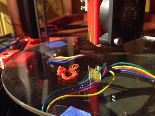
I thought I should give my Kossel a "Robot" page, since Silas asked what the Kossel was, and I told him, "A 3D Printer," to which my precocious son replied, "No, it's a robot."

A lot of the information here is a copy from my build blog, but I've re-thought it's presentation slightly, since there preexist two build guides for the Kossel.

1. Blokmer's Kossel Mini Build Guide
2. builda3dprinter's Kossel Build Guide

Both are put together by organizations selling Kossel kits. Blokmer's guide is much more detailed and slow paced. Of course, I purchased my ...

This is a continuation of my Robot Metallurgy 101 -- AVR Lesson Journal

• USART_1634 Code Github

I started looking through Newbie Hack's tutorials on AVR trying to work up the energy to tackle First LCD Program . Many don't know this, but I despise workings with LCDs. I think it is two parts, one, I live in a world with high-resolution screens embedded in everything from coffee-machines to toilets . Trying to settle with an old school LCD doesn't cut it for me. Furthermore, wiring a non-serial interface LCD is a ever loving pain.

But looking at the rest of the Newbie Hack ...

Originally posted on www.letsmakerobots.com

This is a continuation of my Robot Metallurgy 101 Lesson Journal .

After I was able to get my motors moving using the SN754410 I became a little obessessed with understanding AVR PWM architecture. There are several tutorials that helped me a lot:

1. Newbie Hack's "Intro to PWM."
2. Newbie Hack's "Control a Servo with PWM."
3. humanHardDrive's " PWM "
4. maxEmbedded's " AVR Timers -- PWM MODE "

In the end, I ripped maxEmbedded code and got my PB3 LED working in about 10 minutes. Then, I spent the next three evenings reading trying to figure out what maxEmbedded's code was ...

Originally posted on www.letsmakerobots.com

UPDATE: August 10th, 2014

I printed a body and added BLE. I'll explain tomorrow after I get some rest, but the BLE was to allow me to test directed locomotion. I've also done some feature testing (load-sharing, charging circuit, "hunger" ADC), the board is actually a good design. Works well.

The BLE is the HM-11, itty-bitty BLE.

My goal is to test the physical and feature designs with the ATtiny84, and when Mr. Bdk6 releases his toolchain for the LPC1114, switch it as the controlling chip.

This is my version of Yahmez' Baby Bot ...

Originally posted on www.letsmakerobots.com

Here are some random notes on working with the HM-10.

1. Working RX/TX LEDs
2. How upgrade the HM-10
3. Pseudo Star-Networking HM-10s

Working RX/TX LEDs

I spent some time trying to find a way to create RX/TX traffic LEDs for the HM-10 breakout. This might be easy for some, but it was a real thinker for me. The HM-10 is TTL, which as it was explained me, means that the line is high while idling and low to represent data. The problem here is the typical LED setup doesn't work. Sadly, this is ...

Originally posted on www.letsmakerobots.com

Kobold Files

Awhile back Sparkfun posted a new product, their MiniMoto breakout board. It breaks out the DRV8830 IC, which is a serially controlled (I2C) H-Bridge. I thought the chip was nifty. A few problems though,

1. Sparkfun's breakout was 25x25mm for one bridge. If I added another and then an Arduino Pro Mini it'd lose smallness.
2. It's $9.95
3. It's not on a purple board :)

So, I set out to make a robot controller with it that was smaller than a Sparkfun breakout. What I ended up with is a little bitch I refer ...

This is a continuation of my Robot Metallurgy 101 -- AVR Lesson Journal

• USART_1634 Code Github

UPDATE: Now with UART(ish)! (3/2/2014)

1. Robot Metallurgy 101: PWM
2. Robot Metallurgy 101: UART

I thought I would journal my work as I begin to venture from the comfortable playground of Arduino C and IDE.

I've tried a few other IDEs and C++ to work with different chips. But each time I realize I don't know enough about C/C++, tool-chains, and workspaces to make a robot with them.

Bdk6 gave me an LCP1114 and I was able to get a blink program ...

Originally posted on www.letsmakerobots.com

ATtiny Bitsy Spider

UPDATE: Added BOM corrections. (Sorry for floating.)

Ok. Here's a finished board I've been working on for a bit.

In essence, it is a BLE node board. It combines an HM-10 board with an ATtiny 85. This board builds off:

1. Bluetooth 4.0 (HM-10)
2. ATtiny 85

The idea of the Bitsy Spider board is diminutive controller node. I wanted it to be cheap and versatile enough to use as a node, but I think the final price is around $11 each.

Here's the ole GitHub:

• ATtiny Bitsy Spider (v.02)

The ...

Originally posted on www.letsmakerobots.com

imagesI guess it's been an I2C weekend. I found these organic light-emitting diode displays (OLED)images imagesat Itead studio for $5. images

imagesNifty little buggers.images

They might be small, but their extraordinary contrast and viewing angle more than make up for it. Plus, I mean, c'mon, they're $5. I will say I was a little annoyed that they operate at 3.3v. And I'm sure this means I'll be making a small little level converter board for them pretty soon. I estimate the converter board would be around $1.25, simagestill a good ...

Originally posted on www.letsmakerobots.com

Code

UPDATE: Added info on making SPI programming jig (makes life a lot easier).

UPDATE: Added ATtiny 84 info (though, the post is meant for the ATtiny 85).

I've been non-traditional microcontroller curious for a bit. Then, I had to put a Digi-Key order together for some real cheap stupid stuff (some SOT-23 N-Channels for the LiPo charger circuit) and I thought, "What the hell, let's order some ATTiny 85s." Being cheap like I am, I ordered SMD:

• ATTiny 85 -- SOIC-8 ($1.25 each)

I then ran over to OSHPark and made a little ...