Ladvien's Lab

Originally posted on www.letsmakerobots.com

I've been working on this one in silence for a bit.

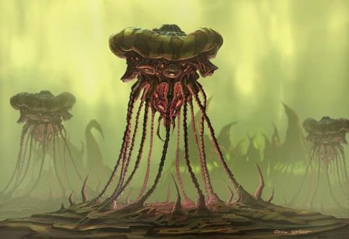
Awhile back it hit me, before I started growing my Overlord project in complexity I wanted to refine it for ease-of-use. Therefore, I began translating my Overlord project into a Python module I could build off.

A Friendly Overlord

I figure, this would make it easier for anyone to use. This includes myself, I've not forgotten my identity as a hack, nor will anyone who pops the hood on this module :)

But, at its core, there are few essential inputs:

1. Color to track ...

Originally posted on www.letsmakerobots.com

I've been working on re-making the the Open Hardware Pulse Sensor so it'd be easy to send off to OSHPark and to make at home. I'm not sure, but I think I started this projects in March and I've just now finished it.

The bit of encouragement I needed was when hackaday.com put it up as their " Fail of the Week. " I thought I was going to be mature about it. But those four red letters started eating at me, so I gave it another go. Weirdly, I got it working.

I believe ...

Originally posted on www.letsmakerobots.com

Videos:

UPDATE: 1/05/13

New angle. I finished my ATtiny Bitsy Spider ( ABS ) board and wanted to do something with it. While stringing it together I had thought of replacing the Arduino Pro Mini and the Servo Helper board with the ABS. Costs wise, it will be slighty more expensive ($1.50 or so?) but much smaller and a lot less hassle.

I've read several people had mixed results getting an ATtiny to control servos. Of course, I'm no better. But I was able to get acceptable functionality out of them (i.e ...

Originally posted on www.letsmakerobots.com

I threw this little guy together for my son Silas because he wanted to play with dad's "Wobot." There's not a lot to say about him, he's a hodgepodge of parts I had lying about:

• HDPE Bought at the Dollar Store for $2 (I guess that's the Two Dollar store.)
• 3-6v 400 RPM Geared Mini Motors: $8
• Two wheels from eBay: $2
• 4-40 bolts, nuts, and washers (local): $4
• Arduino Uno: $9.85
• Ardumoto Shield: $11
• Bluetooth 4.0 Module: $9
• 4 x NiHM lying about: $0
• 1 x Free Sunday morning

Total: $36 ...

Originally posted on www.letsmakerobots.com

NOTE: Try as I might, guys, I can't get the numbers to line up in my HTML version of my code. Instead, you might just load it into Geany or Notepad+ to follow along, since I indicated things by the line number. I'm sorry, I'm out of patience for it.

These are redneck instructions on how to control a robot with a static webcam for under 50 USD.

I'm a robot builder and I got tired of seeing universities play robot soccer or something with computer vision guiding their players, and no matter how ...

Originally posted on www.letsmakerobots.com

• UPDATE: 7/6/14 -- Silkscreen corrections.
• UPDATE: 6/1/14 BOM Corrections.
• UPDATE: 4/2/14 -- Corrected information and linked the new breakout board, v.9.9

Also, this fellow is working on open-source firmware for the HM-10 .

UPDATE (2/514): I split this post, since it's getting a little sluggish.  I've updated the breakout board versioÂn v.9.9, have instructions for updating the firmware, and added some research notes on a pseudo-Star-Network.

• Avandced(ish) HM-10

UPDATE (11/23/13): I've added research notes on networking the HM-10s and an ATtiny 85 serial ...

Originally posted on www.letsmakerobots.com

I'm posting this collection out of frustration and perhaps defeat. I've been working on several projectss for the last two months, trying to finish something. I'd gotten addicted to that "It works!" moment I think anyone gets when they see a LED blink. Sadly, I feel I've failed at most of these projectss.

The second reason I post is posterity.

I've grown to appreciate failure, given how much I learn from it. Of course, I'd much rather learn from other's failures. So, I figure I'd try to write up all my blunders for others ...

Originally posted on www.letsmakerobots.com

UPDATE: I discovered the link I had was referring (which is the true stock image) is unuseable unless update and upgrade are run. Sadly, you can't do that with a 2gb image. Regardless, I've switched the image to the updated (as of writing this) Angstrom image. Please double check and make sure you've got the latest image:

http://beagleboard.org/latest-images

Replace the paths in steps 8 & 10 (but I'll try to keep it up to date). Again, it is unfortunate but you need a 4gb or greater microSD to use these instructions.

**MAIN ...

8/25/13:

This fellow here has made some pretty nifty walkthroughs on the rtl8192 and the Chronodot (DS3231) RTC on the Arch Linux. Though I've not attempted his instructions (been burnt out on this board) I believe his instructions will get a reliable WiFi connection with the rtl8192, using Arch Linux, on the B^3.

• rtl8192 with Arch Linux
• Chronodot (eBay: DS3231 )

Also, when I get the energy, the pinout at the bottom of this page has a mistake or two. As Zaius pointed out.

EDIT: Ok. Don't use the pinout until I research more. I'm getting conflicting information ...

Originally posted on www.letsmakerobots.com

Code

No longer afeared of frying my Pi, I've moved on to trying to implement some of my bot goals. Like many, I want my bot to be able to interact with people, but I didn't realize that I'd stumble on this ability.

I've looked at many visual processing boards like the CMUcam v4 , but I'm not paying $100 for any board. I looked into making one, it looks possible, but not much cheaper. So, I got curious as to what alternatives there are. I stumbled on Hack-a-Day's recommended article: OpenCV on Raspberry Pi ...