Churning Data into Information

I work with a lot of data on the behalf of an agency without a lot of money. Exploring free-to-use and open-source tools is key to being effective in my job.

Recently, I've written a a couple of series on how to use R and SQL to sort through Homeless Management Information System data.

• HMIS, R, and SQL
• HMIS SQL-R Script Snippets

These data are essential to local governments helping individuals experiencing homelessness to be housed quickly and appropriately.

But one area R and SQL have not delivered is on-line interactive dashboards. Data is one thing, but easy to digest information is really key to informing stakeholders how the system is working to end homelessness.

In other projects I've attempted to generate graphs as images and upload to a static link. Then, each time the data change re-generate replace the image. But, most website servers cache the images so it is not ideal.

This has pushed me to try to learn D3.

• D3.js

I'm not going to lie, I've felt confused by languages, IDEs, and libraries. And I've overcome most of the these challenges. But I've never been so confused as by the layout and syntax of D3. The dyslexic feeling I get trying to work in D3 has discouraged me from spending too much time on it.

But recently I decided to take another stab at it-- this time I lucked out and found the C3.js.

• C3.js

Essentially, C3 is a library which greatly simplifies D3. It boils down building a graph into a set of options passed to the C3 graph builder as a JSON object.

This code:

var chart = c3.generate({
    data: {
        x: 'Date',
        y: '# Individuals',
        xFormat: '%Y-%m-%d',
        url: 'https://ladvien.com/projects/d3/data/trendsInTX601.csv',
        type: 'line',
        // colors: {
        //     Count: '#990000'
        // }
        names: {
            NumberHomeless: "Homeless",
            NumberInRRH: "Rapid Rehousing",
            NumberInPSH: "Permanent Supportive Housing"
        }
    },

    title: {
        text: "Homeless or Formerly Homeless in TX-601"
    },

    legend: {
        show: true
    },

    axis: {
        x: {
            type: 'timeseries',
            tick: {
                count: 4,
                format: '%Y-%m-%d',
                // rotate: 90,
                multiline: false,

                culling: {
                    max:5 
                }
            }
        },
        y: {
            max: 3000,
            min: 0,
            label: "# Individuals"
            // Range includes padding, set 0 if no padding needed
            // padding: {top:0, bottom:0}
        },
    },

    point: {
        r: 0
    }
});

Using this CSV:

• trendsInTX601.csv

Produces the following graph:

One Hiccup

I did run into a one hiccup in setup. It seems the most recent version of d3 (version 4.0) has had much of its API overhauled. In such, it will not work with C3. But D3 v3 is still available from the D3 CDN:

<script src="https://d3js.org/d3.v3.min.js"></script>

Calling this library and following the instructions outlined by the C3 site, you can be generating graphs in little time.

• C3 -- Getting Started

Updating Data Securely and On Schedule

Now that I've the ability to use R and SQL to sort through my data, and I could quickly generate graphs using D3 and C3, it'd be really nice if a lot of this could be automated. And luckily, I'd run into a few other tools which made it pretty easy to replace the data on my C3 graphs.

Rsync

Rsync is primarily a Linux tool, but it is available on Windows as well. It is nice since it will allow you to quickly reconcile two file-trees (think of a manual Dropbox).

It will also allow you to sync a local file tree with a server file tree across an SSH connection. For example, I use the following command to sync the data mentioned above to the server

rsync -avz /Users/user/data/js-practice/d3/* ladvien@ladvien.com:/usr/share/nginx/html/projects/d3/

After running this command it will prompt for a password to access the server. Then, it will proceed to sync the two file-trees. Nifty!

This allows me to quickly update the data on the graph. Now, if only there were a way to automatically insert my password, then I could write a script to automate the whole process.

Python Keyring

Python Keyring is a tool which allows you to save and retrieve passwords from your PC's keyring.

• Python Keyring

It is compatible with:

• Mac OS X Keychain
• Freedesktop Secret Service (requires secretstorage)
• KWallet (requires dbus)
• Windows Credential Vault

If you have Python installed you can install the Keyring tool with Pip:

$pip install keyring

After, you can store a password in the keyring by using the command-line tool. You will need to replace username with the name of your server login.

$keyring set system username

And retrieve it with:

$keyring get system username

This is great. It means we can store our password in the keyring and retrieve it securely from a script.

Great! Now we could write a script to have Rsync sync the any data changes locally with the server. Right? Well, almost. We needed one more tool.

SSHPass

There is a problem with using Rsync to sync files remotely from a script. When Rsync is called from a script it will not wait for parameters to be passed to the tool. Sigh.

Luckily, I'm not the only with this problem and a tool was created to solve this problem.

• SSHPass

If you are on a Mac you'll need to use Brew to install SSHPass.

brew install https://raw.githubusercontent.com/kadwanev/bigboybrew/master/Library/Formula/sshpass.rb 

There we go! Now we can automate the whole process.

I wrote this script to do the dirty work:

#!/bin/sh
PASSWORD=("$(keyring get system ladvien.com)")
ECHO ""
ECHO "****************************"
ECHO "* Updating D3 Projects     *"
ECHO "****************************"
ECHO ""
sshpass -p "$PASSWORD" rsync -avz /Users/user/data/js-practice/d3/* root@ladvien.com:/usr/share/nginx/html/projects/d3/

Cron

Ok! One last bit of sugar on this whole process. Let's create a Cron job. This will run the script in the background at an interval of our choosing.

For me, I've a staff who pulls data and runs a master script every Monday. So, I'll set my automated script to update my C3 graph data on Tuesday, when I know new data is available.

• How to Create a Cron Job on a Mac

You can use Nano to edit your Cron job list.

env EDITOR=nano crontab -e

To run a Cron job on Tuesday we would set the fifth asterisk to 2.

* * * * 2 /the/path/to/our/update_script.sh

And don't forget to make the update_script.sh executable.

chmod +x update_script.sh

I'm a hacker hacking with a hacksaw!

I bought a few Raspberry Pi Zero W's for $10. It was happenstance I also purchased the Udemy course Learn Ethical Hacking from Scratch. I figure, I might as well put these things together.

• Raspberry Pi Zero W
• Learn Ethical Hacking from Scratch

I also discovered the Sticky Fingers Kali Pi kernel and distros put together by Re4son.

• Kali Pi

It has worked well so far. However, I've not fully tested the Bluetooth LE hardware on the custom kernel.

One of the issues I've had is not being able to connect to new hotspots headlessly. Usually, you'd boot the rp0w connected to a monitor, keyboard, mouse, and edit wpa_supplicant.conf directly. But what if you want to go into a new location with only your laptop and the rp0w. How would you add the wifi credentials to the rp0w without a monitor, etc.

For awhile, I tried to get the ethernet gadget setup to work on the rp0w without any luck. I think the problems relates to trying to use the gadget hardware on a Mac rather than a Windows machine.

In the end, I decided I would add a script which would do the following:

1. Mount the /boot partition (which is editable through PC's SD card reader).
2. Look for a file on the /boot called "wpa_supplicant.txt" and copy it to the /etc/wpa_supplicant.conf
3. Look for a file on the /boot called "interfaces.txt" and copy it to the /etc/networks/interfaces
4. Unmount /boot
5. Remove the /boot directory

I saved this script in /root as wifi_setup.sh . I then added a call to it in /etc/rc.local

#!/bin/sh -e
#
# rc.local
#
# This script is executed at the end of each multiuser runlevel.
# Make sure that the script will "exit 0" on success or any other
# value on error.
#
# In order to enable or disable this script just change the execution
# bits.
#
# By default this script does nothing.
/root/wifi_setup.sh || exit 1
exit 0

Here's the wifi_setup.sh

#!/bin/bash

if [ ! -d "/boot" ]; then
        echo 'Mounting /boot'
        cd ..
        mkdir /boot
        mount /dev/mmcblk0p1 /boot
fi

if [ -f "/boot/wpa_supplicant.txt" ]; then
        echo 'Applying wpa_supplicant'
        cp /boot/wpa_supplicant.txt /etc/wpa_supplicant.conf
        mv /boot/wpa_supplicant.txt /boot/wpa_supplicant.applied.txt
fi

if [ -f "/boot/interfaces.txt" ]; then
        echo 'Applying intefaces'
        cp /boot/interfaces.txt /etc/network/interfaces
        mv /boot/interfaces.txt /boot/interfaces.applied
fi

umount /boot
rm -r /boot

This has let me add a new network from my laptop with merely an SD card reader.

Creating a Data Error Report by User

In this work challenge we will combine Client and Enrollment data, then we will add a non-HMIS dataframe which contains user account information. After these data are merged, we will then parse them for missing data elements and provide a by-user list of data errors.

Data Needed

As stated above, the data needed are:

1. Client.csv
2. Enrollment.csv
3. A dataframe containg HMIS user contact info.

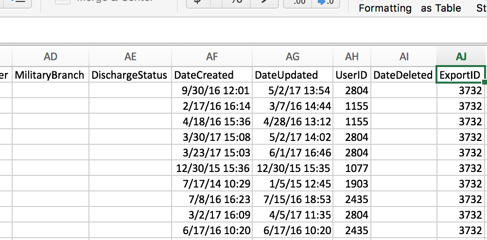
The key to this challenge literally is at the end of every HMIS CSV. Each exported CSV contains some metadata which describes how the data were produced.

The DateCreated should represent when the respective row was actually entered into the HMIS. DateUpdated is the last time that row was modified and saved in the HMIS. The UserID is the case-manager who last modified these data. Lastly, the ExportID is the number which identifies a collection of HMIS CSVs to be in the same batch.

We are going to focus in on the UserID element. Notice, you will not find the usernames, real names, email address, or really any contact information for individual HMIS users. However, having a unique user ID in each CSV would still allow HUD to use internal validity tests to determine the reliability of the user.

For us, we are going to take another source of data containing all of the UserIDs and contact information for the users. Now, this will probably be different each HMIS software vendor. But each vendor should have a way to export a list of the users in the system with their UserID , which will allow us to join these data to the HMIS CSVs.

For those participating in the work challenge from my CoC, I'll provide a CSV with these user data.

After actual user names are joined to the CSVs, then we will begin to parse the CSVs for data errors. If you aren't yet familiar with the term parse in computer science, think of it as diagraming a setence where we make the computer do all the work. Instead of a sentence, we will be diagraming a row of data to determine if there are any errors.

What's an HMIS Data Error?

The HMIS Data Dictionary is specific about what a data error is.

• 8 -- Client doesn’t know
• 9 -- Client refused
• 99 -- Data not collected
• Blank
• Incomplete response
• Non-determinable response

Here's an example of a Client.csv which contains one of each type of error.

Here are the data errors:

1. Tesa is first name blank
2. Sarah's DOB is blank
3. Fela's SSN is an incomplete response (must be 9 digits)
4. Sarah's SSN is non-determinable
5. Sarah's DisablingCondition was not collected.
6. Tesa refused to provide a VeteranStatus.

The Goal

We are going to take a HMIS data and join it with a dataframe containing end-user information. Then, we will create a query to subset the dataframe so we get a dataframe which contains only rows with data errors. Lastly, we will get counts of the types of data errors and the names end-users who've caused the most data errors.

The data elements we will look into for errors:

1. FirstName
2. LastName
3. DOB
4. VeteranStatus
5. DisablingCondition
6. RelationshipToHoH

To get this information we will need to do the following:

1. Load Client.csv, Enrollment.csv, and Users.xlsx
2. Left join the clientDf and enrollmentDf.
3. Left join the usersDf to the result of step 2.
4. Parse the data elements listed above for data errors
5. Create a dataframe which contains only rows with data errors
6. Use the SQL Count function to count the number of data errors by the element list above.
7. Use the SQL Count function to count how many times a end-users name is associated with a row containing errors.
8. Create a dataframe of these counts
9. Save the dataframe containing the error counts into an Excel file (.xlsx)

The Resources

Below are the resources which should help for each step:

TBD

We've worked a bit with Comma Separated Values ( .csv ) files, but it they aren't the only way to store data. There are a lot of data storage formats, each with its strengths and weaknesses. One of the deficits of the CSV format is it cannot store formatting or graphs. This is the reason Excel format ( .xls or .xlsx ) has become another industry standard.

Excel is a program created by Microsoft to allow people to easily work with spreadsheets. With it, they created a way of storing data which allows for formatting and other information to be included. In fact, Excel documents have become so sophisticated programmers can include entire programs within the document. This is the reason you'll often get the "Enable Content" button when open Excel document. That means there is some code embedded in the Excel document which will run if you say "Enable". (Be careful, malicious programmers can insert code which could royally blink up your computer.)

When working with HMIS data being able to load and write Excel documents is necessary. Unfortunately, it adds a lot of complexity.

There are several R libraries which will allow us to work with Excel documents in R. They have different strengths, therefore, I'll focus on two libraries, rather than one.

• XLConnect
• openxlsx

Installing R Libraries for Excel

Installing either of these libraries should be as simple as running the following code:

install.packages("XLConnect", dependencies=TRUE)
install.packages("openxlsx")

However, there are lots of ifs . Both of these libraries rely on the rJava library. Unfortunately, there is often some mismatch of computer architecture. What does that mean? Well, often you'll install R for amd64, but rJava is easiest to get working with R for i386.

Just know, RStudio has a way to set the version of R you are using by going to Tools then go to Global Options . If you are in Windows, at the top of the R General section you will see the option to change your R version. If you are having difficulty getting the above Excel documents working, try switching the R version to i386. (Don't forget to restart RStudio after switching.)

Past this, I'd be more than happy to help you troubleshoot. Just leave a comment below or shoot me an email. However, it can get pretty hairy--especially on a Mac.

Working with XLConnect

Now days, I only use XLConnect to load data from Excel sheets. I've just been too lazy to re-write all my code to use one library (which would be openxlsx ). It's my opinion the reason to use XLConnect is it's a little easier to understand how it loads data. Its weakness is it doesn't have as much flexibility in formatting Excel documents to be saved on your computer. And it can be confusing to save Excel sheets.

Loading Data from Xlsx Documents

Loading data using XLConnect is a little different than using the read.csv function. Like I stated earlier, Xlsx documents contain other information besides data. One critical piece of information is the sheet number.

Unlike CSVs a single Excel document can contain multiple spreadsheets. Each of these sheets will be broken out in tabs when you open an Excel document

XLConnect doesn't make any assumptions, it wants you to tell it which sheet you'd like to load.

Here's how to load an Excel document, the first sheet, in XLConnect:

library(XLConnect)
excelDf <- readWorksheetFromFile("/Users/user/Data/VI-SPDAT v2.0.xlsx", sheet = 1, startRow = 1)

It is similar to the read.csv() function, but notice the file in the path refers to VI-SPDAT v2.0.xlsx ? You want to make sure your file format is either .xlsx or .xls as the readWorkSheetFromFile() function only works with Excel documents.

Also, there are two other parameters. The first, sheet = 1 is telling XLConnect to read in only the first sheet. Just know, you could set it to whatever sheet number you'd like. And for reference, the sheets are 1, 2, 3, 5...etc., left to right when opened in Excel. So, even if your sheets have different names XLConnect will still load the data respective to their numerical order.

The second parameter is startRow = 1 . This allows you to tell R where to start the dataframe. For example, if you had a header in your Excel document which didn't contain data.

We could skip down to row three, where the column headers are, by telling XLConnect startRow = 3 .

Writing a Dataframe to Excel Document

Writing Excel documents are a little more complex--and one reason I'm not a huge fan of XLConnect.

Here's how you'd write an Excel file:

######################### Data ###################################
###################### DO NOT CHANGE #############################
peopleDf <- data.frame(PersonalID=c("ZP1U3EPU2FKAWI6K5US5LDV50KRI1LN7", "IA26X38HOTOIBHYIRV8CKR5RDS8KNGHV", "LASDU89NRABVJWW779W4JGGAN90IQ5B2"), 
                       FirstName=c("Timmy", "Fela", "Sarah"),
                       LastName=c("Tesa", "Falla", "Kerrigan"),
                       DOB=c("2010-01-01", "1999-1-1", "1992-04-01"))
##################################################################
##################################################################

# Create a workbook to contain the worksheet(s).
peopleWorkbook <- loadWorkbook("People.xlsx",  create = TRUE)
# Create and name the worksheet.
myPeopleWorksheet <- createSheet(peopleWorkbook, "My People")
# Add the data to the worksheet, put it in the workbook, save it to the computer.
writeWorksheetToFile("People.xlsx", data = peopleDf, sheet = "My People")

After running this code you should have a file called People.xlsx in your working directory (remember, getwd() will tell provide the working directory). If you open this file, it should look something like this:

This looks a little complex, but it's just because XLConnect makes it look complex. Here's what it is is doing:

1. A workbook is created, which is a place where worksheets can be stored.
2. myPeopleWorksheet is created inside the workbook created above. The sheet is called "My People"
3. The worksheet has our peopleDf added to it, then it is saved as a file called "People.xlsx" in our working directory.

Like I said, it's a lot of unneeded complexity, in my opinion.

Why use Excel Documents

After the added complexity of reading and saving Excel documents you might wonder what the benefit is? Great question.

As stated at the beginning, Excel documents can contain other information besides just data. It contain formatting, images, graphs, and a lot of other stuff. And one of the reasons for writing report scripts is to automate all redundant tasks.

Imagine, you've got a data set of 12,000 participant enrollments. You want to create a spreadsheet which puts the enrollment in descending order. And you want to create this report daily.

If you used the write.csv() you would need to open the CSV after creating it, then manually add the sort to the document, save it as an Excel file, then send it out. I guarantee, after doing that for several weeks you are going to want to find a way to automate it. Especially, if you decide the headers need to have font size 18 as well.

Excel documents allow us to store the formating tweaks and XLConnect allows us to insert them automatically.

Adding formatting can get a little more complex and will be the focus of another article. Also, we will use openxlsx as it is much easier to output formatting, again, just my opinion.

Comparative Functions

Comparing two or more values is an extremely important concept when talking to computers. In writing a report script, it is is essential. Comparisons allow us to filter to values within a range, allowing us to provide a report of relevant information.

Take the following data:

######################### Data ###################################
###################### DO NOT CHANGE #############################
peopleDf <- data.frame(PersonalID=c("ZP1U3EPU2FKAWI6K5US5LDV50KRI1LN7", "IA26X38HOTOIBHYIRV8CKR5RDS8KNGHV", "LASDU89NRABVJWW779W4JGGAN90IQ5B2"), 
           FirstName=c("Timmy", "Fela", "Sarah"),
           LastName=c("Tesa", "Falla", "Kerrigan"),
           DOB=c("2010-01-01", "1999-1-1", "1992-04-01"))
##################################################################
##################################################################

If you run the above in R you should get a dataframe called peopleDf which looks like this:

It's a simple table. But let's say we wanted to get a list of everyone born before 2000-01-01. Of course, we can easily see Timmy is the only person born after 2000. But if our table was thousands of records it wouldn't be possible to quickly assess.

Luckily, this is pretty straight forward in SQL-R. We will use a less than operator ( < ). You probably remember this sign from high-school while solving inequalities. However, we will be using it as what's known as a relational operator .

In short, it states,

Is x less than y

If x is less than y the computer is going to say the statement is true (or 1 in binary). If it is not, then the computer will say it's false (or 0 in binary). Believe it or not, this simple operation is why you have a device in your pocket which could calculate the internal mass of the sun.

For us, things are a little simpler. We just want to know who was born before 2000. Let's re-write the statement above with our problem:

Is Sarah's DOB less than 2000-01-01

Well, what is Sarah's DOB? 1992-04-01. Let's rewrite and assess (gah, this feels like high-school algebra again).

Is 1992-04-01 less than 2000-01-01

Hmm. This can get confusing for humans, but more importantly, confusing to computers.

In English, we'd probably state this as,

Did 1992-04-01 come before 2001-01-01?

Essentially, that's what we are doing. Just know, the computer will translate all dates into a number. This number is how many seconds transpired since 1970-01-01.

Why? On Thursday, January 1st 1970 the Universal Coordinated Time (UTC) was established. Think of it is when the world came together to standardize time. Computer people figured, "Well, if we have to convert dates into a raw number for computers to understand it, it might as well be the number of seconds since UTC was established."

Ok, enough history lesson. How is this relevant?

1. Computers convert dates into seconds since 1970-01-01.
2. Comparing dates is actually comparing numbers.

Taking our statement again, let's re-write it with the number of seconds since 1970-01-01

Is number of seconds between 1970-01-01 and 1992-04-01 less than number of seconds between 1970-01-01 and 2000-01-01

Which becomes:

Is 702,086,400 less than 46,684,800 seconds

Aha, now this makes sense. And the result is true . We can now say, in computer speak: Sarah was born before 2000-01-01 .

Why? Really, dude.

In my world there is a saying: RFTM .

It's hard to follow now days. Everything moves quick and we don't have time to dig into the "Why." But, like most things, if you want to be good, you must take the time to do so.

The reason we review how computers understand dates is it directly impacts how we write reports. Do you remember the date conversion trick to get dates to work in SQL from R? This is because R holds dates as the number of seconds since 1970 and passes it as a string to SQL. But, then SQL tries to convert the date from a date into seconds again, screwing everything up.

It pays to RFTM.

Filtering Dataframes by Date

Back to the problem. How do we write a script which provides a dataframe of people born before 2000-01-01?

The code is actually pretty simple,

library(sqldf)
nonMillennialsDf <- sqldf("SELECT * FROM peopleDf WHERE DOB < '2000-01-01'")

This should provide a nonMillennialsDf dataframe, which contains:

And there we go, for all my nerdsplaining the code's pretty simple, right?

Well, there are a few gotchas. Notice the date we've written. It has the following format YYYY-MM-DD and is surrounded by single quotes. Any time you use dates in SQL they must be written in this format.

Another tricky part is trying to find if a date falls between two dates. Let's take the peopleDf and write a query which provides everyone who was born between 1998-01-01 and 2005-01-01

Here's the query.

bornBetweenDf <- sqldf("SELECT * FROM peopleDf WHERE DOB > '1998-01-01' AND DOB < '2005-01-01'") 

This should result in a table with only Fela:

It is important to understand, the first comparison removed Sarah, as 1992-04-01 is less than 1998-01-01 . Then, the second comparison got rid of Timmy as 2010-01-01 is greater than 2005-01-01 .

Now()

There is one more critical command in writing robust date comparisons. The NOW() function. This function is different in R and SQL, but pretty much every programming language has a version of the function.

Essentially, the NOW() asks the computer what today's date is when the script runs.

In SQL-R it looks like this:

nowDf <- sqldf("SELECT *, DATE('NOW') As 'TodaysDate' FROM peopleDf")

This should provide:

And it doesn't matter when this script is run, it will always insert today's date in the TodaysDate column. Nifty, right? Trust me, if you don't see the possibilities yet, give it time. It'll grow into one of your favorite functions.

Well, we can't talk about the NOW() function without discussing the DATE() function I slipped in there. What does it do?

As we discussed earlier, the computer looks at dates as the number of seconds since 1970-01-01 . When you use the NOW() function by itself then it will return the number of seconds--um, not something humans like to read. The DATE() function says, "Take whatever is inside the parentheses and try to convert it into a human readable date." Voila! A human readable date.

Age

Let's get fancy. We can use the NOW() function and our peopleDf to calculate everyone's age.

peopleWithAgeDf <- sqldf("SELECT *, (DATE('NOW') - DOB) As 'Age' FROM peopleDf")

This should provide:

Cool, right? Now, it does not matter when this above code of line is run, it will calculate everyone's age correctly.

One important note, if the date and time are wrong on your computer this calculation will be incorrect.

The nerd-judo which can be done with dates in SQL-R is endless. But this covers a lot of the basics.

If you've missed the code bits throughout this article, here it is all at once:

######################### Data ###################################
###################### DO NOT CHANGE #############################
peopleDf <- data.frame(PersonalID=c("ZP1U3EPU2FKAWI6K5US5LDV50KRI1LN7", "IA26X38HOTOIBHYIRV8CKR5RDS8KNGHV", "LASDU89NRABVJWW779W4JGGAN90IQ5B2"), 
           FirstName=c("Timmy", "Fela", "Sarah"),
           LastName=c("Tesa", "Falla", "Kerrigan"),
           DOB=c("2010-14-01", "1999-1-1", "1992-04-01"))
##################################################################
##################################################################
library(sqldf)
nonMillennialsDf <- sqldf("SELECT * FROM peopleDf WHERE DOB < '2000-01-01'")
bornBetweenDf <- sqldf("SELECT * FROM peopleDf WHERE DOB > '1998-01-01' AND DOB < '2005-01-01'") 
nowDf <- sqldf("SELECT *, DATE('NOW') As 'TodaysDate' FROM peopleDf")
peopleWithAgeDf <- sqldf("SELECT *, (DATE('NOW') - DOB) As 'Age' FROM peopleDf")

Providing Chronically Homeless List

With this work challenge we are going to take the concepts we've learned from the first challenge and build on them. We will combine two dataframes derived from Client.csv and Enrollment.csv. Then, we will apply HUD's formula to get a by-name-list of those who are chronically homeless.

Data Needed

The current definition of chronically homeless is found in HUD's federal register :

A “chronically homeless” individual is defined to mean a homeless individual with a disability who lives either in a place not meant for human habitation, a safe haven, or in an emergency shelter, or in an institutional care facility if the individual has been living in the facility for fewer than 90 days and had been living in a place not meant for human habitation, a safe haven, or in an emergency shelter immediately before entering the institutional care facility. In order to meet the “chronically homeless” definition, the individual also must have been living as described above continuously for at least 12 months, or on at least four separate occasions in the last 3 years, where the combined occasions total a length of time of at least 12 months. Each period separating the occasions must include at least 7 nights of living in a situation other than a place not meant for human habitation, in an emergency shelter, or in a safe haven.

There are several data elements which will be needed for us to calculate whether someone is chronically homeless. These data elements are reported to case-managers and entered into a HUD Entry Assessment when a client enters a program.

Here's a list of the data elements we will use:

1. DisablingCondition
2. TimesHomelessPastThreeYears
3. MonthHomelessPastThreeYears
4. DateToStreetESSH

All of the above data elements are found in the Enrollment.csv. Therefore, similar to the last Challenge, we will need to join the Client.csv and the Enrollment.csv.

We've covered how to get all data from CSVs into one dataframe using joins. This Challenge will build on that skill. The new concepts here will be combining logic to get to a specific answer.

• Logic

In SQL we will use the following logic operators:

• IS (==)
• NOT (!=)
• AND (&&)
• OR (||)
• > (greater than)
• < (less than)

For example, let's take the chronically homeless definition and turn it into something a computer can understand using these logic operators. We can do this by re-writing the definition several times, each time dropping what makes sense to humans and leaving what makes sense to computers.

For example, this should make sense to most humans.

A chronically homeless individual is disabled and been homeless greater than 364 days. Or, is disabled and been homeless greater than three times in three years and the time spent in homelessness adding up to greater than 364 days.

That paragraph seems a little hard to read, right? But still, humans should be able to understand it. Now, let's look at the same paragraph emphasizing the logic operators.

A chronically homeless individual IS disabled AND been homeless GREATER THAN 364 days. OR , IS disabled AND been homeless GREATER THAN three times in three years AND the time spent in homelessness adding up to GREATER THAN 364 days.

This is skill of a Computational-Thinker, taking a definition like HUD provided and re-write it from something a human would understand into something a computer will understand.

The next step is re-writing the paragraph in something called pseudo-code .

Chronic Homeless Individual == 

                    A person IS Disabled AND
                    A person > Homeless 364 days

                    OR

                    A person IS Disabled AND
                    A person homeless > 4 times AND
                    A person > 12 months homeless within 3 years

This helps us make sure everything is in place to feed to the computer. The next step will be actually writing the SQL code.

Below is the following code to get chronically homeless:

#############################################
##### Get those with Disabling Condition ###
#############################################
disablingCondition <- sqldf("SELECT PersonalID 
                            FROM clientAndEnrollmentDf 
                            WHERE DisablingCondition = 1")

#############################################
##### Length-of-Stay ########################
#############################################
# Participants who meet the length-of-stay in homelessness requirement
# Either through four or more occurences with cumulative duration exceeding a year
# Or a consequtive year.
#                 113 = "12 Months"
#                 114 = "More than 12 Months"
chronicityDf <- sqldf("SELECT PersonalID, 'Yes' As 'Meets LOS'
                               FROM activeEnrollment
                               WHERE (TimesHomelessPastThreeYears = 4
                                    AND (
                                          MonthsHomelessPastThreeYears = 113
                                          OR MonthsHomelessPastThreeYears = 114)
                                        )
                               OR (CAST(JULIANDAY('now') - JULIANDAY(DateToStreetESSH) AS Integer) > 364
                                   AND (DateToStreetESSH != '') 
                                  )
                               ")

#############################################
##### Chronically Homeless ##################
#############################################
# Take the distinct PersonalIDs of individuals who meet both chronicity
# and disabling condition.
chronicallyHomeless <- sqldf("SELECT DISTINCT(a.PersonalID)
                              FROM chronicityDf a
                              INNER JOIN disablingCondition b
                              ON a.PersonalID=b.PersonalID
                             ")

This may look overwhelming, but that'll be the purpose of this week's Challenge, to demonstrate this is code is actually pretty simple when broke down into its basic parts.

That's the real lesson here, every complex question may be made extremely simple when taken once piece at a time. The power of computational-thinking is extraordinary.

The Goal

We are going to merge the two data sets and to discover the following:

1. A list of individuals who are chronically homeless.
2. Export this list to an Excel document.

To get this information we will need to do the following:

1. Load the Client.csv into the dataframe clientDf.
2. Load the Enrollment.csv into the dataframe enrollmentDf.
3. Inner join the clientDf to enrollmentDf.
4. Calculate whether someone is chronically homeless.
5. Filter to those who are chronically homeless.
6. Write the by-name-list of individuals to an Excel document.

The Resources

Below are the resources which should help for each step:

Step 1 & 2

• R Programming A-Z -- Video 41 -- Loading and Importing Data in R
• R Programming A-Z -- Video 21 -- Functions in R
• Read and Write CSVs in R

Step 3

• The Complete SQL Bootcamp -- Video #51 -- Overview of Inner Joins
• The Complete SQL Bootcamp -- Video #52 -- Example of Inner Joins * HMIS, R, SQL -- Basics

Step 4 & 5

• HMIS, R, SQL -- Queries
• HMIS Data Dictionary
• Query Results Using Boolean Logic (all sections and videos)

Step 6

• Writing Excel Workbooks -- Tutorial Coming

I'm fat. Fatter than I want to be. I've not always been fat, I got down to 180 at back in 2008. It took counting calories and weight religiously. The key piece for me was having a graph which I looked at daily showing my outcomes. Over the course of a year I lost 40 pounds. Well, it's time to do it again. I've gained that 40 back over 10 years--and now it needs to go.

Back in 2008 I was using Google to give me the calories of every item I ate and recording them in an Excel document. This food journal was great, but a little more work than it probably should have been.

Back then, I wasn't aware of being a hacker. Now, I plan to throw all my hacker skills at this weight loss plan (hell, I might even go to the gym!)

I signed up for MyFitnessPal. Counting calories worked once, I figure if it aint broke. But then I got to looking at how much work it would take to look at my improvement. I mean, I'd have to actually open the app on my phone and click on the weight loss section. Shesh--who designed that app? Two actions to get where I needed--ain't no one got time for that.

Enter hacker skills. I discovered there is a Python library which allows scraping of data.

• MyFitnessPal Python Library

This wonderful little library is written and provided by CoddingtonBear.

I figure, I'd write a Python script to scrap the data, save it to a CSV, create an SQL-R script to join the nutrition and weight information, use ggplot to plot the data, save the plot as a PNG, and then copy this plot to a dedicated spot on Ladvien.com. Lastly, I'd write a bash script to run every night and update the graph. Simples!

And c'mon, opening a webpage is a lot easier than tapping twice.

Well, after a few hours of coding, I've got the first step of the project complete.

import myfitnesspal
import csv, sys, os
from datetime import datetime

# Get account info
client = myfitnesspal.Client('cthomasbrittain')
# Set start year
startYear = "2008"
# Get limits
beginningDate = datetime.strptime(startYear, "%Y").date()
beginningYear = beginningDate.year
daysInMonth = {1:31, 2:28, 3:31, 4:30, 5:31, 6:30, 7:31, 8:31, 9:30, 10:31, 11:30, 12:31}
emptyNutrition = [None, None, None, None, None, None]

print("")
print("################################################")
print("# Scraping MyFitnessPal                        #")
print("# Make sure your account is set to public      #")
print("# and your username and pass are in keychain   #")
print("################################################")
print("")

today = datetime.now().date()
currentYear = today.year

print("")
print("################################################")
print("# Get nutrition and weight information         #")
print("################################################")
print("")

# Loop over years from beginingYear.  Make sure last year is inclusive.
for yearIndex in range(beginningYear, currentYear+1):

    # Create a file name based on this year's data
    thisFileName = "healthData_%s.csv" % yearIndex

    # Open CSV as read and write.
    # If file exists, open for read / write
    #   else, create file, write only.
    try:
        f = open(thisFileName, "r+")        # Check to see if file is complete,
        row_count = sum(1 for row in f)     # else, overwrite the file
        if(row_count != 366):               # A year of rows plus headers, and an empty line at end.
            f = open(thisFileName, "w+")
            row_count = 0
    except EnvironmentError:
        f = open(thisFileName, "w+")        # If file does not exist, create it.
        row_count = 0

    writer = csv.writer(f)

    # Check number of lines. If the year wasn't captured, start over.
    if(row_count < 365):
        # Write headers for totals
        writer.writerow(["Date", "Sodium", "Carbohydrates", "Calories", "Fat", "Sugar", "Protein", "Weight"])
        sys.stdout.write(str(yearIndex)+": ")   # Print has a linefeed.
        sys.stdout.flush()
        for monthIndex in range(1, 12+1):

            beginningOfMonthStr = "%s-%s-%s" % (yearIndex, monthIndex, 1)
            endOfMonthStr = "%s-%s-%s" % (yearIndex, monthIndex, daysInMonth[monthIndex])

            beginningOfMonth = datetime.strptime(beginningOfMonthStr, "%Y-%m-%d").date()
            endOfMonth = datetime.strptime(endOfMonthStr, "%Y-%m-%d").date()

            thisMonthsWeights = dict(client.get_measurements('Weight', beginningOfMonth, endOfMonth))

            for dayIndex in range(1, daysInMonth[monthIndex]+1):

                fullDateIndex = "%s-%s-%s" % (yearIndex, monthIndex, dayIndex)
                thisDate = datetime.strptime(fullDateIndex, "%Y-%m-%d").date()
                if(thisDate > today):
                    break;

                thisDaysNutritionData = client.get_date(yearIndex, monthIndex, dayIndex)
                thisDaysNutritionDataDict = thisDaysNutritionData.totals
                thisDaysNutritionValues = thisDaysNutritionDataDict.values()

                thisDaysWeight = [(thisMonthsWeights.get(thisDate))]

                if(len(thisDaysNutritionValues) < 6):
                    thisDaysNutritionValues = emptyNutrition

                dataRow = [fullDateIndex] + thisDaysNutritionValues  + thisDaysWeight
                if dataRow:
                    writer.writerow(dataRow)

            sys.stdout.write("#")
            sys.stdout.flush()
        print(" -- Done.")
        f.close()
    else:
        print((str(yearIndex)+": Exists and is complete."))

And then we add some R to join the data together and automate plotting, and saving the plots as images.

library(ggplot2)
library(scales)

cat("*******************************************************\n")
cat("* Starting R                                          *\n")
cat("*******************************************************\n")
cat("\n")
cat("*******************************************************\n")
cat("* Combining Health Data                               *\n")
cat("*******************************************************\n")
cat("\n")
# Thanks Rich Scriven
# https://stackoverflow.com/questions/25509879/how-can-i-make-a-list-of-all-dataframes-that-are-in-my-global-environment
healthDataRaw <- do.call(rbind, lapply(list.files(pattern = ".csv"), read.csv))
# Fill in missing values for calories
healthDataRaw$Calories[is.na(healthDataRaw$Calories)] <- mean(healthDataRaw$Calories, na.rm = TRUE)

date30DaysAgo <- Sys.Date() - 30
date90DaysAgo <- Sys.Date() - 90
date180DaysAgo <- Sys.Date() - 180

cat("*******************************************************\n")
cat("* Creating Weight Graph                               *\n")
cat("*******************************************************\n")
healthData <- healthDataRaw[!(is.na(healthDataRaw$Weight)),]
healthData$Date <- as.Date(healthData$Date)
healthData <- with(healthData, healthData[(Date >= date30DaysAgo), ])
p <- ggplot(healthData, aes(x = Date, y = Weight))+
  geom_line(color="firebrick", size = 1) +
  labs(title ="Ladvien's Weight", x = "Date", y = "Weight")
p
ggsave("ladviens_weight.png", width = 5, height = 5)

cat("\n")

cat("*******************************************************\n")
cat("* Creating Calories Graph                             *\n")
cat("*******************************************************\n")
cat("\n")
#healthData <- healthDataRaw[!(is.na(healthDataRaw$Calories)),]
healthData$Date <- as.Date(healthData$Date)
healthData <- with(healthData, healthData[(Date >= date30DaysAgo), ])
p2 <- ggplot(healthData, aes(x = Date, y = Calories))+
  geom_line(color="firebrick") 
p2

png(filename="ladviens_calories.png")
plot(p2)
dev.off()

cat("*******************************************************\n")
cat("* Finished R Script                                   *\n")
cat("*******************************************************\n")
cat("\n")

Lastly, let's write a bash script to run the Python and R code, then copy the images to Ladvien.com

#!/bin/sh
PASSWORD=("$(keyring get system ladvien.com)")

Python myfitnesspall_scraper.py

Rscript myfitnesspal_data_sort.R

ECHO ""
ECHO "*******************************************************"
ECHO "* Syncing files to Ladvien.com                        *"
ECHO "*******************************************************"
ECHO ""

# Used SSHPass
# https://gist.github.com/arunoda/7790979

sshpass -p "$PASSWORD" scp ladviens_weight.png ladviens_calories.png root@ladvien.com:/usr/share/nginx/html/images/

And here's the result:

My weight:

And my calories:

Next, I'll probably tweak ggplot2 to make the graphs a little prettier. Also, I'll setup a Raspberry Pi or something to run the bash script once a night. Why? Lolz.

Enrollment.csv

Many of the CSVs in the HMIS CSV may contain multiple rows per client. This can make it difficult when working with HMIS data, as it appears to the non-data person there are duplicates within your data.

Let's look at some dataframes:

enrollmentDf

Notice how Bob has two records? One on 10/17/2016 and 01/01/2013. This represents two HUD Entry Assessments completed on Bob. These HUD Entry Assessments could represent two stays in the same program, or one stay in two programs.

Regardless, whenever you go to join this dataframe with a another dataframe, like the Client.csv, it will cause the resulting dataframe to have two rows representing both of Bob's enrollments.

Let me walk us through joining the above dataframe with another dataframe.

We are going to join the enrollmentDf (above) with this clientDf

enrollmentDf

clientDf

In R, we can join these two dataframes with the following.

Please copy the code below to R and execute.

####### BEGIN LOADING DATA FRAMES ###############
enrollmentDf = data.frame(ProjectEntryID=c("L0TDCLTDEARVHNIQ4F9EDDKXJ764Z65Q", "169ACC89JY5SX0U87U7HQ28PMMHNJEXQ", "XB52BYOGJ1YDFESNZVNGDGA58ITDML0A"), 
               PersonalID=c("ZP1U3EPU2FKAWI6K5US5LDV50KRI1LN7", "IA26X38HOTOIBHYIRV8CKR5RDS8KNGHV", "ZP1U3EPU2FKAWI6K5US5LDV50KRI1LN7"), 
               FirstName=c("Bob","Jane", "Bob"), 
               EntryDate=c("10/17/2016", "05/05/2015", "01/01/2013"))

clientDf = data.frame(PersonalID=c("ZP1U3EPU2FKAWI6K5US5LDV50KRI1LN7", "IA26X38HOTOIBHYIRV8CKR5RDS8KNGHV"), 
                      FirstName=c("Bob","Jane"),
                      LastName=c("Beber", "Goodall"))
####### ENDS LOADING DATA FRAMES ###############

# Load the SQLdf package (note, it must be installed first. See install.packages())
library(sqldf)

# Join the two dataframes.
clientAndEnrollmentDf <- sqldf("SELECT * 
                               FROM clientDf 
                               LEFT JOIN enrollmentDf 
                               ON clientDf.PersonalID=enrollmentDf.PersonalID")

Important Sidenote

If you ever see the following error:

In field_types[] <- field_types[names(data)] : number of items to replace is not a multiple of replacement length

It's a problem with going back-and-forth between R and SQL. To fix it, use the following code on the dataframe you are trying to work with before executing the line of code causing the error

dfCausingProblem <- subset(dfCausingProblem)

Ok, back to work.

After executing the code, you should end up with a table like this. Not too shabby.

However, notice there are still rows for Bob? These aren't technically duplicates. A duplicate is when there are two rows where items in every column are exactly the same. But in the case of the dataframe above, notice how the ProjectEntryID and EntryDate columns for Bob's records are different?

As stated before, this is carried forth from Bob having two HUD Entry Assessments. But to the people whom we are going to present these data, it looks like duplicates. This is a problem because it will be seen as sloppy work (but remember, it's not. It's merely a technical artefact).

Who cares! How do we get rid of it?

First, we have to make a decision among three options. First, we can get only the most HUD Entry Assessment per client, only the the first HUD Entry Assessment ever taken per client, or leave it as it is.

The last option is out, so it's a choice between most recent and the oldest one. In our world, homelessness usually gets worse and HUD wants us to be helping those who are the most vulnerable first, so the most recent is probably going to give us the best picture how vulnerable a client is right now.

Alright, how do we get the most recent HUD Assessment?

In SQL there is a function called MAX() . It will take the most recent of a record. Let's look at how to use it, then we can discuss it.

For the following code to work, make sure all code above has been executed in R.

clientAndEnrollmentDf2 <- sqldf("SELECT *, MAX(EntryDate) FROM clientAndEnrollmentDf")

This should provide you with the following table:

Wait! What happened to Jane!? Well, the MAX() took the row with the greatest EntryDate, which is 10/17/2016. Unfortunately, Jane's record wasn't the most recent, so her record was removed.

Well, that's not going to work. But we're close. If only we had a way to take the MAX(EntryDate) per client.

We do. SQL has another command called GROUP BY, which allows us to tell SQL to apply another command by a group of records.

Again, let's use it and then dissect it.

Copy this to R and execute it.

clientAndEnrollmentDf3 <- sqldf("SELECT *, MAX(EntryDate) FROM clientAndEnrollmentDf GROUP BY PersonalID")

You should end up with a table like this:

Aha! That's it!

What the GROUP BY did was say, "Ok, SQL, create a group of data where the rows PersonalID are the same. Now, for each group, take the row with the greatest EntryDate."

This gives exactly what we want. A single row per participant.

R let's us work with HMIS data, but there is still the problem of how to load the data into R from a source. R is actually pretty neat regarding data importing. We can load data from a website, SQL database, text file, Excel file, or CSV.

When working with HMIS data the two most common types of data source are Excel and CSV. Therefore, it's going to pay to spend a little time on how to bring those files into R.

Importing CSVs into R

CSV stand for Comma Separated Value format. It is a near ancient file format which is used to store data in rows and columns. If you have a CSV file on the computer (in Windows) right-click on it and open it in Notepad. The contents should look something like this:

PersonalID,FirstName,LastName
B7YIOJIGF9CDP6FV7TANQXLMQRMBTVTB,Bob,Person
ASGJ4F95HS85N39DJ12AJB094M59DJ45,Jane,People

However, if you open the same CSV in Excel it will look something like this:

Let's be honest, the second example is easier for humans to read (well, unless you're an odd human). And for the most part, we will be looking at CSVs in Excel or in RStudio's dataview which looks similar to Excel. However , it is important to note the easier to read version can hide data errors that may only be visible by viewing the raw CSV. Nothing to worry about now, but keep it in mind.

Alright, let's explore how to load a CSV file into R. There is many way's to do this, but let's start with a super-easy way:

r pathToCsv <- file.choose() myCsvAsADataFrame <- read.csv(pathToCsv)

These two commands, when executed, will force R to create a file selection box. This will allow us to easily select the CSV to load into R. Once selected and we press Ok then R will load the selected file's path into the variable pathToCsv .

The next command read.csv() takes the path provided and attempts to load the file it points to and converts it into a dataframe. Once R creates a dataframe from the file selected it saves it in the variable myCsvAsADataFrame

And that's it. The data is now loaded into R and it can be manipulated with other commands.

Writing CSVs

Saving data from R is the other end of importing data. This process is often referred to as exporting data. Really, it's simply taking a R dataframe and converting it into a file--once in a file form it can be loaded into Excel or emailed to a peer (but, please don't email personal information--remember, CSVs are simply text).

To write data a CSV use write.csv() .

For example:

write.csv(theDataFrameToWrite, "NameOfFile.csv")

That's it, pretty simple, eh? Well, there are a couple of catches. When R saves a CSV it does a few things which are annoying for using the data in other way. For example, let's say we have data in R that looks like this:

However, after it is written to a file it will look like this:

Note the added NA . It is a good practice to put an NA in places where there are no data. Unfortunately, when dealing with HMIS data sets the standard is to leave a blank instead. To get R to conform to this standard we use an option in the write.csv() function.

For example:

write.csv(theDataFrameToWrite, "NameOfFile.csv", na="")

The na="" tells R to write the document without changing blanks into NA . The result of the code above should look like:

Mixing R and SQL is powerful. One of the easiest ways to implement this combination is with the R library SQLdf.

If TL;DR, skip to Coerce Date Types into Strings before Passing to SQLdf at bottom.

SQLdf

The power of SQLdf comes from its ability to convert dataframes into SQLite databases on the fly. To the user, it doesn't appear like anything special is going on, but under the hood R is working together with a SQLite client to create a table which can be queried and manipulated with ANSI SQL calls.

For example,

dataFrame1 <- read.csv(pathToData)
library("sqldf")
dataFrame2 <- sqldf("SELECT FirstName FROM dataFrame")

These three lines do a lot. It loads data from a CSV, loads a library of functions for convert R dataframes into SQLite databases, and then the sqldf() function call does two things at once. It converts the R dataframe into a SQLite database and then queries it for the FirstName column.

If we were to assume the dataFrame1 variable contained data like this:

Then the dataFrame2 <- sqldf("SELECT FirstName FROM dataFrame) will create a variable called dataFrame2 which contains the FirstName column from dataFrame1

And this is how we will shape our data in the R-SQL way.

Datatypes

One of the most important things a human can learn about computers is something called datatypes. When computers process information they need a little help from humans in attempt to understand what to do with the information. For example, what do these numbers mean to you?

76110, 444-325-7645, 10/24/1980

Most humans (at least in the United States) will know the first number is a ZIP code, the second a phone number, and last date. Humans know this because our brains have learned how to discern from context. In the case of the ZIP code, it's exactly 5 numbers, the phone contains dashes at at exact places, and the date contains slashes in the exact spot we'd expect of a date.

Unfortunately, computers have a little more difficulty with this. Most computers are smart enough now days to know the phone number and date of birth, but the ZIP code will confuse the heck out of a computer.

A computer's initial reaction in seeing the ZIP code is, "Oh, you mean 76,110. That's a big number." When really, this number represents a geographic location.

Ok, let's make this more relevant to HMIS work. The way to help a computer understand what numbers are representing is by telling the computer what type of data a particular column is. This is known as a datatype. For us, we really only deal with a few datatypes, but their are hundreds of thousand of datatypes.

In R you can see what datatype a column of your dataframe is by clicking the blue button next to the dataframe name in the Global Environment variables.

We will be dealing with the following:

• Dates (called "POSXct" in R)
• Strings (called "chr" in R)
• Numbers
• Factors

Of course, every programming language can calls these datatypes by different names, thus, furthering confusion. (I mean, c'mon, programming is simple enough as it is--we've got to make it a little challenging.)

Dates

Date datatypes usually look like this:

10/24/1980

But it can come in many different formats. It's probably best to differentiate between datatype and data format . A data type describes how the information should be used--it's important for a computer. Data format describes how a computer should display information to the human--therefore, it's useful for a human.

An example of different formats of the same data:

10/24/1980
1980-10-24
102480

Ok, back to the date datatype. It is used when dealing with dates. By declaring a variable as having a date datatype, it is telling the computer whatever we put into that variable to interpret as a date. Simple enough.

Strings

When we talk about string we aren't talking about fuzzy things kittens chase. A string datatype is a series of characters (one part of a string) strung together. Anything can be a string. They are probably the most important datatype, since they can tell a computer to look at a number and see something else. Confused? Let's look at some examples.

We tell a computer data is a string is by putting it in double quotes "this is a string" or single quotes 'this is also a string' .

Here's an example of assigning a string in R:

myFirstString <- "this is a string"

Great! But what can we do with it? Well, a lot.

Let's say we wanted to pass a path of a file to a read.csv() function. We could do so by providing the path as a string.

dataFrame <- read.csv("/Users/user/Downloads/Client.csv")

The above will load the Client.csv file located at the /Users/user/Downloads/ directory--the computer knows how to read the path because it's a string.

But why are strings so important? Well, they allow us to tell a computer to override its basic instinct and view a piece of data as something other than what the computer would guess it is.

Returning to the ZIP code.

notAZipCode <- 76110
myZipCode <- "76110"

These variable assignments may seem to be exactly the same, however, the first one creates a variable as a number, but the second tells the computer, "This is a not a number, it is something else--please don't pretend to understand it. I'll tell you exactly what to do with it later."

Numbers

Number datatypes are easy. It's pretty much how a computer tries to look at all data you provide it. One important characteristic about numbers, you can have the computer perform math functions on numbers, which you couldn't on strings.

dataframe1 <- 12 * 12 
datafram2 <- "12" * "12"

Above, dataframe1 will contain 144 after being executed. But if the second line is attempted to be executed the computer will freak out, "This is a string! I can't add strings! You told me you'd tell me what to do with them..."

Factors

Factors are a special datatype in R. Most of all the variables we load in R will start out as factors. Essentially, factors are categories of data.

Red,
Orange,
Green,
Blue,
Indigo,
Violet

Is an example of factors. They are categories of data. The important of factors will become more evident as we work through these tutorials in R.

If you don't understand factors, it's cool. Just think of them as strings. However, if you don't understand strings, please ask any questions in comments below. Understanding them is critical to working with SQLdf.

SQLdf and Datatypes

Anytime you mix two different languages it pays to be careful about meaning. As I learned once by talking about pie as something I liked--come to find out, it was funny to Hispanic friends who were learning English. (Apparently pie is Spanish for foot?)

When mixing R and SQL we must be careful about how the two languages look at the datatypes. In R it sees dates as a POSXct datatype (this is essentially fancy date datatype. Would you like to know more ?)

Well, this is all fine and dandy, but when we pass commands from R to SQL it is all passed as a string.

dataFrame2 <- sqldf("SELECT * FROM dataFrame1")

Notice SELECT * FROM dataFrame1 is all in quotation marks? This turns it into a string then it passes it SQLite, which is hidden to us.

If all this is a bit overwhelming, no worries. Bookmark this page to refer back to later. Just remember the following:

Date columns must be converted into a chr datatype before passing it to SQL. How to we convert datatypes? It's pretty darn simple. We use something called data coercion.

Coercing Data Types

Let's go back to that ZIP code and number example. Let's say the computer reads all your ZIP codes from a file as a number. This happens a lot, since to the computer that's what it looks like--so it guesses that's what you are going to want.

But no, we want those ZIP codes to be strings. To do this, we can get a particular column from a dataframe by writing the name of the dataframe then $ then the name of the column. For example, datafram$zipCodes will return only the column zipCodes from dataframe.

Alright, now we have a way to select one column from our dataframe we can attempt to convert that one column's datatype. To do this use the as.character() command.

dataframe$zipCodes <- as.character(dataFrame$zipCodes)

This will convert the zipCode column from a number into a string, then, it assigns it back to the column zipCodes. Boom! We've told the computer to stop trying to make a ZIP code a number. Instead, treat it as a string. And with that, we will tell the computer later how to use ZIP codes.

Coerce Date Types into Strings before Passing to SQLdf

Ok, now for the reason for this entire article. Before passing any dates to SQLdf we need to first convert them to strings. Otherwise, SQLdf will try to treat them as numbers--which will cause a lot of heartache.

For example, a Client.csv file should have a DateCreated column. This represents the date a case-manager put the data into HMIS. The data should look something like this:

Let's try to get all of the clients who've been entered after 10/01/2014.

dataFramContainingDates <- read.csv("/Users/user/Downloads/Client.csv")
datesEntered <- sqldf("SELECT * FROM dataFramContainingDates WHERE DateCreated > '2014-10-01'")

The above code should provide every column where DateCreated date is greater than 2014-10-01. But, instead, it will result in an empty dataframe. Waaah-waah.

Essentially, this is because SQL is comparing a number and a string. It freaks the computer out.

Instead, we should convert the DateCreated column to a string instead of a date. Then, SQL will actually convert it from a string to a date.

Confused? Imagine me when I was trying to figure this out on my own.

Ok, so, the take away? Before passing any dates to SQL convert them to strings.

dataFramContainingDates <- read.csv("/Users/user/Downloads/Client.csv")
dataFrameContaingDates$DateCreated <- as.character(dataFrameContaingDates$DateCreated)
datesEntered <- sqldf("SELECT * FROM dataFramContainingDates WHERE DateCreated > '2014-10-01'")

By using the as.character function to convert the DateCreated column to a string and then assigning it back to the dateframe, it sets SQL up to do the date comparisons correctly. Using the dateframe from above, this should result in the following table:

Confused as heck? Feel free to ask questions in the comments below!