This post shows how to setup a Raspberry Pi 3B+ for operating a Tensorflow CNN model using a Pi Camera Module v2.0 .

Raspberry Pi Setup

I will be focusing on the Raspberry Pi 3B+, but don't worry if you are using a different Pi. Just let me know in the comments below and I'll try to get instructions for your particular Pi added.

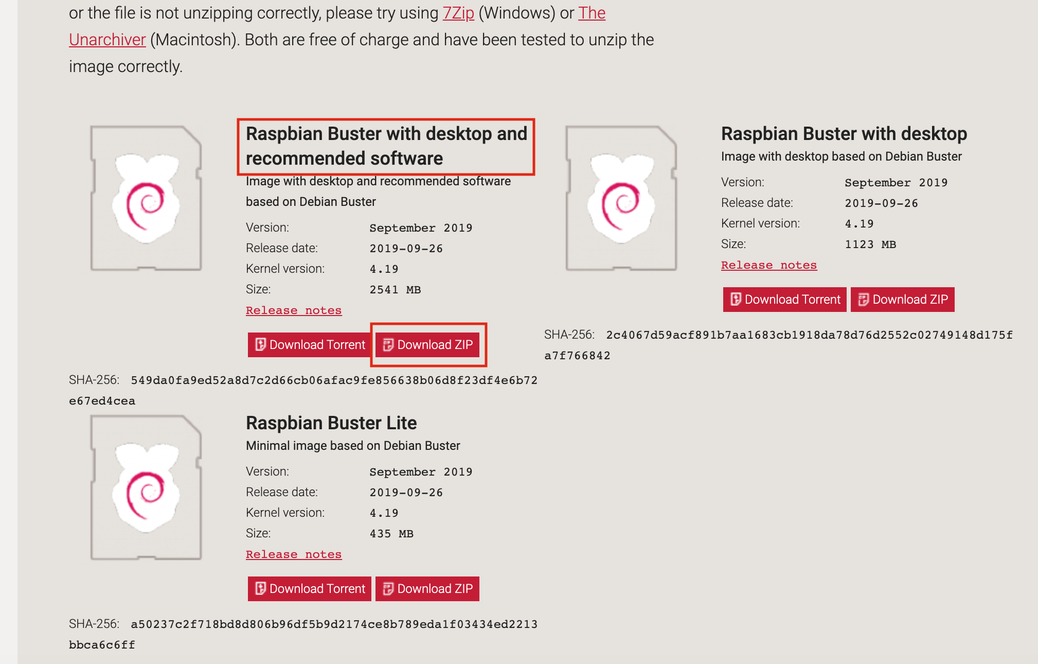
Step #1: Download Raspbian Buster with desktop and recommended software

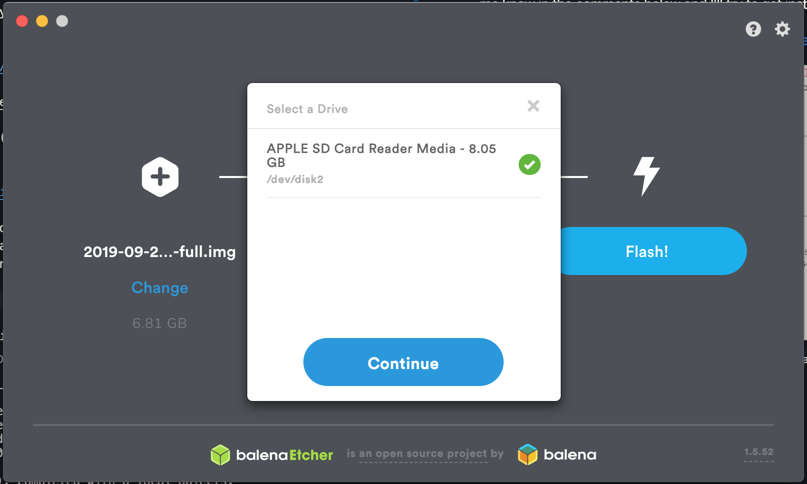
Step #2: Write the image to a 8gb (or greater) SD card. I use Etcher .

Step #3: Once the image is finished, and before you plug the card into the Pi, open the SD card and create a file called ssh . No extension and nothing inside. This will enable ssh on boot.

Step #4: Plug the card in to the Pi. Step #5: Plug a LAN cable into the Pi Step #6: Attach your PiCam.

Note, there are two plugs the PiCamera will mate with. To save frustration:

Step #7: Turn the Pi on. Step #8: Find the ip of your Pi and ssh into it with the following.

ssh pi@your_pi_ip

The password will be raspberry

The easiest way to find your Pi's ip is to login into your router. Usually , you can login into your router by opening a webbrowser on your PC and typing 192.168.1.1 . This is the "home" address. You should then be prompted to login to the router. On your router's web interface there should be a section for "attached devices." You can find your Pi's ip there. If many are listed, you can turn off your Pi and see which ip goes away. That was probably the Pi's ip.

Step #9: Once on the Pi, run the following

sudo raspi-config

This should open a old school GUI.

Enable the following under Interfacing Options

Camera
VNC

The camera will allow us to use the PiCamera and VNC will allow us to open a a remote desktop environment, which should make it easier to adjust the PiCamera.

(Optional) When working with a remote desktop environment, too high of a resolution can cause responsiveness issues with the VNC client (RealVNC). To prevent this, the Raspbian setup automatically adjusts the Pi resolution to the lowest. Unfortunately, I find this troublesome when trying to do computer vision stuff from the Pi. The following will allow you to adjust the resolution--just keep in mind, if it's too high there could be trouble. Oh, one note here, this is the main reason I'm using a LAN connection to my Pi, as it allows greater throughput than WiFi.

Update! Apparently, if you raise your Pi's resolution too high, then you will not be able to start your PiCam from Python. This is due to the PicCam buffering frames in the GPU memory of the Pi. Of course, you could increase the GPU's memory through raspi-config (it defaults to 128, max is 256). Of course, then you've less RAM to put in your Tensorflow model.

My opinion, raise the Pi's screen resolution just high enough to make it easy for debugging the Pi cam. And when you get ready to "productionize" your Pi, drop the resolution to the lowest.

Ok, if you still want to, here's how to raise the Pi's resolution.

Still in raspi-config open Advanced Options . Navigate to Resolution and change it to what you'd like. (I'm going with the highest).

Once you've finished setting these options, exit. At the end it will ask if you want to reboot, say "Yes."

Step #10: Download and install RealVNC Viewer .

Step #11: Open RealVNC and set the ip to your Pi. Don't include your user name, like we did when ssh 'ing, because RealVNC is about to ask us for it. Once you've typed in the ip hit "Enter" or "Return."

Step #12: RealVNC will warn you about singing into your Pi, as it's not a credentialed source. No worries. Hit continue.

Note, if you're on a Mac, it's going to ask you to give RealVNC access to keys or something. (Shesh, Mac, thank you for the security, but, well, shesh.)

Step #13: Enter your credentials.

username: pi
password: raspberry

Step #14: This should open your Pi's desktop environment. It will ask you a few setup questions, go ahead and take care of it. Note, if you change your password, you will need to update RealVNC (if you had it "Remember My Password").

Tensorflow Setup

Here's where it gets real.

Open terminal, either in the VNC Pi desktop, or through ssh . Then enter the following commands.

pip3 install pip3 install https://github.com/lhelontra/tensorflow-on-arm/releases/download/v1.14.0-buster/tensorflow-1.14.0-cp37-none-linux_armv7l.whl

The above installs a Tensorflow 1.14 for Python 3.7.x on the Raspberry Pi 3b+ from ihelontra 's private Tensorflow ARM builds. I've found this better, as Google seems to break the installs often.

If you want another combination of Tensorflow, Python, and Pi, you can see ihelontra 's other whl files:

• tensorflow-on-arm

OpenCV Setup

Tensorflow will allow us to open a model, however, we will need to feed the model image data captured from the PiCamerae. The easiest way to do this, at least I've found so far, is using OpenCV .

Of course, it can be tricky to setup. The trickiest part? If you Google how to set it up on Raspberry Pi you will get tons of misinformation . In all due fairness, it once was good information--as you had to build OpenCV for the Pi, which took a lot of work. But, now days, you can install it using the build in Linux tools.

Ok, back at the Pi's command prompt:

# Install OpenCV
sudo apt-get install python3-opencv

At of time writing, the above command will install OpenCV 3.2. Of course, the newest version is 4.0, but we don't need that. Trust me, unless you've a reason to be using OpenCV 4.0 or greater, I'd stick with the Linux repos. Building OpenCV can be a time consuming pain.

There's one other handy package which will make our work easier: imutils .

Let's install it.

pip3 intall imutils

Using Tensorflow to Classify Images on an RPi.

Now the payoff.

I've prepared a Python script which loads a test model, initializes the Pi camera, captures a stream of images, each image is classified by the Tensorflow model, and the prediction is printed at the top left of the screen. Of course, you can switch out the entire thing be loading a different model and corresponding json file containg the class labels (I've described this in an earlier article .)

Let's download the script and test our build:

cd ~
git clone https://github.com/Ladvien/rpi_tf_and_opencv
cd rpi_tf_and_opencv

Ok! Moment of truth. Let's execute the script.

python3 eval_rpi.py

If all goes well, it will take a minute or two to initialize and you should see something similar to the following:

Troubleshooting

If you are using a different PiCamera module than the v2.0 you will most likely need to adjust the resolution settings at the top of the script:

view_width               = 3280
view_height              = 2464

If you clone the repo in a different directory besides the /pi/home directory, then you will need to change the model path at the top of the file:

model_save_dir           = '/home/pi/rpi_tf_and_opencv/'

Any other issues, feel free to ask questions in the comments. I'd rather troubleshoot a specific issue rather than try to cover every use case.

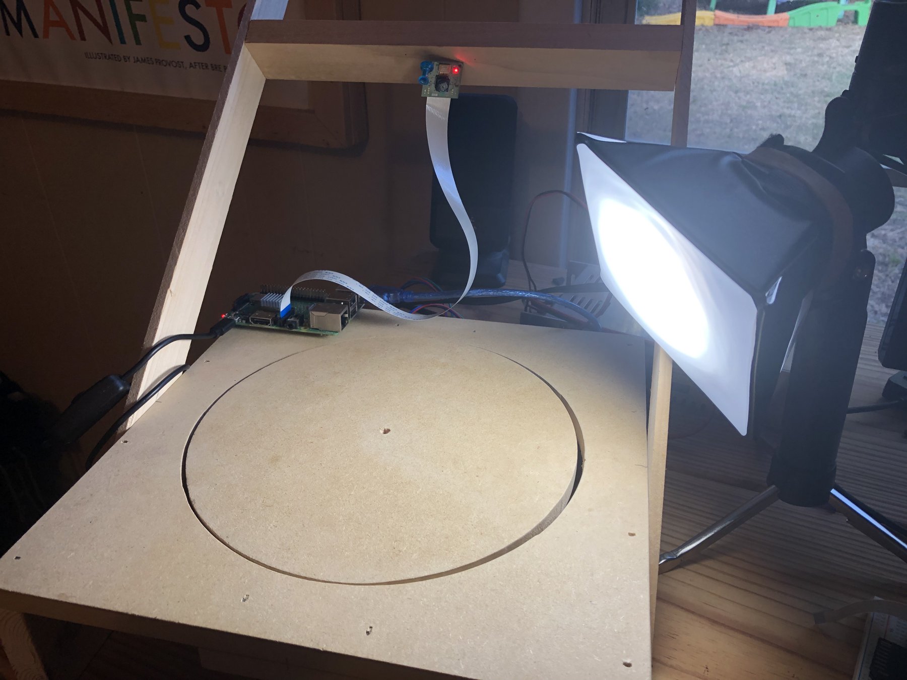
After having success with training a CNN on our initial dataset, we decided to up the game on generating training images. My buddy Rockets built a nice little turntable and ordered a couple of NEMA17s for each of us. His idea was we could both start generating training images.

I asked if he would be OK with me ordering some RAMPs boards and programming them to synchronize with the PiCamera. I figured, it would probably be better for reproducibility if we had solid hardware, with custom firmware and software.

After a few hours of coding over a couple of weeks I was able to control the RAMPs within a Python script from either the Raspberry Pi or a desktop computer.

• Turn Table Controller Code

I've listed the code parts below with a brief explanation--just in case someone would like to hack them for other projects.

Minimum Viable Hack

Warning words, I'm an advocate of the minimum viable product, especially, when it comes to my personal hacking time. I refer to this as the minimum viable hack. That stated, there are known issues in the code below. But! It does the job--so I've not addressed them.

Here are a few: 1. The value 0x0A ( \n ) value is not handled as part of packet (e.g., if MILLI_BETWEEN = 10 bad things will happen). 2. The motors are always on (reduces motor life). 3. Pulse width is not adjustable without firmware update. 4. The Python code is blocking. This makes the halt feature on the Arduino Mega side fairly useless. 5. Only RAMPs motor X is setup (this one I will address later, as we will need several drivers before the end of this project).

RAMPS Code

To move the turn table we used a RAMPs 1.4 board:

• RAMPS Kit (Amazon)

Getting things going was straightforward. I put together the hardware, installed the Arduino IDE, and looked-up the pinout for the RAMPs controller.

I wrote the firmware to receive serial commands as a packet. The packet structure (at time of writing) looks like this:

MOTOR_PACKET = 0x01 0x01 0x00 0x03 0xE8 0x05 0x0A
INDEX        =  1    2     3    4    5    6   7
 ```
* `first_byte` = This indicates what sort of packet type.  Right now, there is only one, but I figure we might want to control other I/O on the Arduino later.
* `second_byte` = the motor selected 1-5 (X, Y, Z,  E1, E2).
* `third_byte` = Motor direction, `0x00` is clockwise and `0x01` is counter-clockwise.
* `fourth_byte` = first chunk of the steps.
* `fifth_byte` = second chunk of the steps.  The steps variable tells the motor how many steps to move before stopping.
* `sixth_byte` = delay between steps in milliseconds.
* `seventh_byte` = the end-of-transmission (EOT) character.  I've used `\n`.

When the code receives an EOT character, it parses the packet and calls the `writeMotor()`.  This function loops through the number of steps, delaying between each.  Each loop, the function checks if a `halt` command has been received.  If it has, it stops the motor mid-move.

Again, this code isn't perfect.  Far from it.  But it does the job.

```cpp
#include <avr/interrupt.h> 
#include <avr/io.h> 
// https://reprap.org/mediawiki/images/f/f6/RAMPS1.4schematic.png
// https://reprap.org/forum/read.php?219,168722

// TODO: Pulse width set by initialization.
// TODO: Setup all motors to be selected by master.
// TODO: Add a timer to shutdown motors after threshold.
//       And keep motor enabled until threshold has been met.
// TODO: Handle 0x0A values as part of packet (e.g., if MILLI_BETWEEN = 10).
// TODO: Add a "holding torque" feature; making it so motors never disable.

// For RAMPS 1.4
#define X_STEP_PIN         54
#define X_DIR_PIN          55
#define X_ENABLE_PIN       38
#define X_MIN_PIN           3
#define X_MAX_PIN           2

#define Y_STEP_PIN         60
#define Y_DIR_PIN          61
#define Y_ENABLE_PIN       56
#define Y_MIN_PIN          14
#define Y_MAX_PIN          15

#define Z_STEP_PIN         46
#define Z_DIR_PIN          48
#define Z_ENABLE_PIN       62
#define Z_MIN_PIN          18
#define Z_MAX_PIN          19

#define E_STEP_PIN         26
#define E_DIR_PIN          28
#define E_ENABLE_PIN       24

#define SDPOWER            -1
#define SDSS               53
#define LED_PIN            13

#define FAN_PIN            9

#define PS_ON_PIN          12
#define KILL_PIN           -1

#define HEATER_0_PIN       10
#define HEATER_1_PIN       8
#define TEMP_0_PIN         13   // ANALOG NUMBERING
#define TEMP_1_PIN         14   // ANALOG NUMBERING

#define MOTOR_X         0x01
#define MOTOR_Y         0x02
#define MOTOR_Z         0x03
#define MOTOR_E1        0x04
#define MOTOR_E2        0x05

#define DRIVE_CMD       (char)0x01
#define HALT_CMD        (char)0x0F
#define DIR_CC          (char)0x00
#define DIR_CCW         (char)0x01

#define COMPLETED_CMD   (char)0x07
#define END_TX          (char)0x0A
#define ACK             (char)0x06 // Acknowledge
#define NACK            (char)0x15 // Negative Acknowledge


// Determine the pulse width of motor.
#define MOTOR_ANGLE           1.8
#define PULSE_WIDTH_MICROS    360 / MOTOR_ANGLE

#define RX_BUFFER_SIZE 16

/*
  MOTOR_NUM:
      X     = 0
      Y     = 1
      Z     = 2
      E1    = 3
      E2    = 4

  PACKET_TYPES
      0x01 = motor_write
      0x02 = motor_halt

  DIRECTION
      0x00 = CW
      0x01 = CCW

  MOTOR MOVE PROTOCOL:
                       0               1     2     3        4       5         6
  MOTOR_PACKET = PACKET_TYPE_CHAR MOTOR_NUM DIR STEPS_1 STEPS_2 MILLI_BETWEEN \n
  MOTOR_PACKET =    01                01    00    03     E8        05         0A
  MOTOR_PACKET =    0x 01010003E8050A

  HALT         = 0x0F
*/


/* Create a structure for the motors
 *  direction_pin = pin to control direction of stepper.
 *  step_pin      = pin to control the steps.
 *  enable_pin    = pin to enable motor.
 */
struct MOTOR {
  uint8_t direction_pin;
  uint8_t step_pin;
  uint8_t enable_pin;
  uint8_t pulse_width_micros;
};

struct BUFFER {
  uint8_t data[RX_BUFFER_SIZE];
  uint8_t bufferSize;
  uint8_t index;
  boolean packetComplete;
  uint8_t shutdownThreshold;
};

/* Initialize motors */
MOTOR motorX = {
      X_DIR_PIN,
      X_STEP_PIN,
      X_ENABLE_PIN,
      PULSE_WIDTH_MICROS
};

// Urgent shutdown.
volatile boolean halt = false;
volatile static bool triggered;

/* Initialize RX buffer */
BUFFER rxBuffer;;



/* Initialize program */
void setup()
{
  Serial.begin(115200);

  // Initialize the structures
  motorSetup(motorX);
  rxBuffer.bufferSize = RX_BUFFER_SIZE;

  // Disable holding torque.
  digitalWrite(motorX.enable_pin, HIGH);
}

/* Main */
void loop()
{
  // If packet is packetComplete
  if (rxBuffer.packetComplete) {

    uint8_t packet_type = rxBuffer.data[0];

    switch (packet_type) {
      case DRIVE_CMD:
        {
          // Unpack the command.
          uint8_t motorNumber =  rxBuffer.data[1];
          uint8_t direction =  rxBuffer.data[2];
          uint16_t steps = ((uint8_t)rxBuffer.data[3] << 8)  | (uint8_t)rxBuffer.data[4];
          uint8_t milliSecondsDelay = rxBuffer.data[5];

          // Let the master know command is in process.
          sendAck();

          // Start the motor
          writeMotor(motorX, direction, steps, milliSecondsDelay);
        }
        break;
      default:
        sendNack();
        break;
    }
    // Clear the buffer for the nexgt packet.
    resetBuffer(&rxBuffer);
  }
}


/*  ############### MOTORS ############### */

/* Method for initalizing MOTOR */
void motorSetup(MOTOR motor) {

  // Setup motor pins
  pinMode(motor.direction_pin, OUTPUT);
  pinMode(motor.step_pin, OUTPUT);
  pinMode(motor.enable_pin, OUTPUT);

}

/* Write to MOTOR */
void writeMotor(MOTOR motor, int direction, uint16_t numberOfSteps, int milliBetweenSteps) {

    // Enable motor.
    digitalWrite(motor.enable_pin, LOW);

    // Check direction;
    switch (direction) {
      case DIR_CC:
        digitalWrite(motor.direction_pin, HIGH);
        break;
      case DIR_CCW:
        digitalWrite(motor.direction_pin, LOW);
        break;
      default:
        sendNack();
        return;
    }

    // Move the motor (but keep an eye for a halt command)
    for(int n = 0; n < numberOfSteps; n++) {
      // Interrupt motor
      if(checkForHalt()) {  
        sendAck();
        break; 
      }
      digitalWrite(motor.step_pin, HIGH);
      delayMicroseconds(motor.pulse_width_micros);
      digitalWrite(motor.step_pin, LOW);
      delay(milliBetweenSteps);
    }

    // Disable holding torque.
    digitalWrite(motor.enable_pin, HIGH);

    // Let the user know the move is done.
    sendCompletedAction();
}

// END MOTORS

/*  ############### COMMUNICATION ###############
 * 
*/
void serialEvent() {

  // Get all the data.
  while (Serial.available()) {

    // Read a byte
    uint8_t inByte = (uint8_t)Serial.read();

    // Store the byte in the buffer.
    rxBuffer.data[rxBuffer.index] = inByte;
    rxBuffer.index++;

    // If a complete packet character is found, mark the packet
    // as ready for execution.
    if ((char)inByte == '\n') {
      rxBuffer.packetComplete = true;
    }

  }
}

// Clear the buffer.
void resetBuffer(struct BUFFER *buffer) {
  memset(buffer->data, 0, sizeof(buffer->data));
  buffer->index = 0;
  buffer->packetComplete = false;
}

// Does not count termination char.
int packetLength(BUFFER buffer){
  for(int i = 0; i < buffer.bufferSize; i++) {
    if((char)buffer.data[i] == '\n'){ return i; }
  }
  return -1;
}

void sendAck() {
  Serial.write(ACK);
  Serial.write(END_TX);
}

void sendNack() {
  Serial.write(ACK);
  Serial.write(END_TX);
}

void sendCompletedAction() {
  Serial.write(COMPLETED_CMD);
  Serial.write(END_TX);
}

// Halt is handled outside normal communication protocol.
boolean checkForHalt() {
  if (Serial.available()){
    // Halt command has no termination character.
    if ((uint8_t)Serial.read() == HALT_CMD) {
      return true;
    }
  }
  return false;
}

// END COMMUNICATION

Python RAMPS

There are two variants of the Python code. First, is for the Raspberry Pi. It's where I focused coding time, as it made sense to generate training images using the same hardware (PiCamera) as would be used for production. However, I've a simpler desktop version which uses OpenCV and a webcam.

• Raspberry Pi Turn Table
• Desktop Turn Table

For the Raspberry Pi and desktop versions you will need the following: * Python 3.7 -- this should be standard on Raspbian Buster.

On the desktop you will need opencv , it can be installed using:

pip install opencv

In both cases you will need the custom class ramps_control , if you clone the repository and run your script from the ./turn_table directory, that should be handled for you.

What's it Do?

The turn table script initializes the camera. It then creates a loop over the number of angles you want to take images.

A full rotation is 3200 steps and if you ask for 60 images, then the script will rotate the turntable ~ 53.33 steps. At the end of the rotation, the script will capture an image of your target. Then, it will rotate another 53.33 steps and take another picture. It will do this 60 times, where it should have completed a full rotation.

#!/usr/bin/env python3
# -*- coding: utf-8 -*-
"""
Created on Wed Sep 25 05:58:48 2019

@author: ladvien
"""

from picamera import PiCamera
import os
from time import sleep
import ramps_control
import serial
import glob

#################
# Parameters
#################

MILLI_BETWEEN_STEPS     = 5
IMAGES_PER_ROTATION     = 60
FULL_ROTATION           = 3200
STEPS_BEFORE_PIC        = int(FULL_ROTATION / IMAGES_PER_ROTATION)

print(f'Steps per image: {STEPS_BEFORE_PIC}')

####################
# Don't Overwrite
####################
def check_existing_images(output_directory):
    existing_image_files = glob.glob(f'{output_directory}/*.jpg')
    max_file_index = 0
    for file in existing_image_files:
        file_index = file.split('/')[-1].split('_')[1].replace('.jpg', '')
        try:
            file_index = int(file_index)
            if file_index > max_file_index:
                max_file_index = file_index
        except:
            pass
    return max_file_index

#################
# Open Serial
#################
ser = serial.Serial('/dev/ttyUSB0', 115200)
print(ser.name)   

#################
# Init Camera
#################
#picam v2 resolution 3280 x 2464
camera = PiCamera()
PIC_SIZE = 1200
CAM_OFFSET_X = 0
CAM_OFFSET_Y = 0
camera.start_preview()

#################
# Init RAMPS
#################
ramps = ramps_control.RAMPS(ser, debug = False)

# Track whether the motor is at work.
motor_moving = False

# Reset the RAMPs program.
ramps.reset_ramps(False)

#################
# Main
#################

part = ''

while True:
    part_candidate = input(f'Enter part number and hit enter. (Default {part}; "q" to quit): ')

    if part_candidate.lower() == 'q':
        print('Bye!')
        quit()
    elif part_candidate != '':
        part = part_candidate

    output_directory = f'/home/pi/Desktop/lego_images/{part}' 

    if not os.path.exists(output_directory):
        os.makedirs(output_directory)

    max_file_index = check_existing_images(output_directory)

    for i in range(IMAGES_PER_ROTATION):

            success = ramps.move(ramps.MOTOR_X,
                        ramps.DIR_CCW,
                        STEPS_BEFORE_PIC,
                        MILLI_BETWEEN_STEPS)

            if success:
                print('Table move a success.')

                file_path = f'{output_directory}/{part}_{i + max_file_index}.jpg'
                print(file_path)
                camera.capture(file_path)

            # sleep(0.05)

ser.close()
camera.stop_preview()

Python RAMPS Class

To increase resuability of the code, I've abstracted the RAMPs controller code into a Python class. This class is called by the script above. It is blocking code which handles sending commands, polling the Arduino, and reports received information.

#!/usr/bin/env python3
# -*- coding: utf-8 -*-
"""
Created on Sat Sep 28 05:39:18 2019

@author: ladvien
"""
from time import sleep, time


"""
  MOTOR_NUM:
      X     = 0
      Y     = 1
      Z     = 2
      E1    = 3
      E2    = 4

  PACKET_TYPES
      0x01 = motor_write
      0x02 = motor_halt

  DIRECTION
      0x00 = CW
      0x01 = CCW

  MOTOR MOVE PROTOCOL:
                       0               1     2     3        4       5         6
  MOTOR_PACKET = PACKET_TYPE_CHAR MOTOR_NUM DIR STEPS_1 STEPS_2 MILLI_BETWEEN \n

"""

class RAMPS:
    DRIVE_CMD       = 0x01
    HALT_CMD        = 0x0F
    DIR_CC          = 0x00
    DIR_CCW         = 0x01

    COMPLETED_CMD   = 0x07
    END_TX          = 0x0A
    ACKNOWLEDGE     = 0x06
    NEG_ACKNOWLEDGE = 0x15


    MOTOR_X         = 0x01
    MOTOR_Y         = 0x02
    MOTOR_Z         = 0x03
    MOTOR_E1        = 0x04
    MOTOR_E2        = 0x05

    def __init__(self, ser, debug = False):
        self.ser = ser
        self.toggle_debug = debug
        self.rx_buffer_size = 256
        self.serial_delay = 0.1

    def toggle_debug(self):
        self.debug = not self.debug

    def print_debug(self, message):
        if self.toggle_debug:
            print(message)

    """ 
            COMMUNICATION
    """

    # Prepare for a serial send.
    def encode_packet(self, values):
        return bytearray(values)

    # Prepare a packet the slave will understand
    def prepare_motor_packet(self, motor_num, direction, steps, milli_between):
        steps_1 = (steps >> 8) & 0xFF
        steps_2 = (steps) & 0xFF
        return [self.DRIVE_CMD, motor_num, direction, steps_1, steps_2, milli_between, self.END_TX]

    def read_available(self, as_ascii = False):

        self.print_debug(f'Reading available.')

        # 1. Get all available data.
        # 2. Unless buffer exceeded.
        # 3. Return a list of the data.

        incoming_data = []
        incoming_data_size = 0

        while self.ser.in_waiting > 0:
            incoming_data_size += 1

            if incoming_data_size > self.rx_buffer_size:
                self.print_debug(f'Buffer overflow.')
                return list('RX buffer overflow.')

            if as_ascii:
                incoming_data.append(self.ser.readline().decode('utf-8'))
            else:
                incoming_data += self.ser.readline()

        self.print_debug(f'Completed reading available.')
        return incoming_data


    def check_for_confirm(self, command_expected):
        confirmation = self.read_available()
        if len(confirmation) > 0:
            if confirmation[0] == command_expected:
                return True
        else:
            return False


    """ 
            RAMPS UTILITY
    """

    def reset_ramps(self, print_welcome = False):

        self.print_debug(f'Reseting Arduino.')
        # Reset the Arduino Mega.
        self.ser.setDTR(False)
        sleep(0.4)
        self.ser.setDTR(True)
        sleep(2)   

        # Get welcome message.
        welcome_message = []

        while self.ser.in_waiting > 0:
            welcome_message.append(self.ser.readline().decode('utf-8') )

        self.print_debug(f'Completed reset.')
        if print_welcome:
            # Print it for the user.
            print(''.join(welcome_message))
            return
        else:
            return

    """ 
            MOTOR COMMANDS
    """
    def move(self, motor, direction, steps, milli_secs_between_steps):

        # 1. Create a list containg RAMPs command.
        # 2. Encode it for serial writing.
        # 3. Write to serial port.
        # 4. Check for ACK or NACK.
        # 5. Poll serial for completed command.

        packet = self.prepare_motor_packet(motor,
                                           direction,
                                           steps,
                                           milli_secs_between_steps)
        packet = self.encode_packet(packet)

        self.print_debug(f'Created move packet: {packet}')

        self.write_move(packet)

        # Don't miss ACK to being in a hurry.
        sleep(self.serial_delay)
        confirmation = self.read_available()
        if confirmation[0] == self.ACKNOWLEDGE:
            self.print_debug(f'Move command acknowledged.')

        if(self.wait_for_complete(120)):
            return True

        return False

    def wait_for_complete(self, timeout):

        # 1. Wait for complete or timeout
        # 2. Return whether the move was successful.

        start_time = time()

        while True:
            now_time = time()
            duration = now_time - start_time
            self.print_debug(duration)
            if(duration > timeout):
                return False

            if self.check_for_confirm(self.COMPLETED_CMD):
                self.print_debug(f'Move command completed.')
                return True

            sleep(self.serial_delay)

    def write_move(self, packet):        
        self.ser.write(packet)
        self.print_debug(f'Executed move packet: {packet}')

Questions

That's pretty much it. I've kept this article light, as I'm saving most of my free time for coding. But, feel free to ask questions in the comments below.

This article is part of a series. It should explain the code used to train our convolutional neural-network (CNN) LEGO classifier.

If you want to code along with this article, we've made it available in Google's Colab:

• Lego Classifier

Or if you want to run the code locally:

• lego_sorter

It's a WIP, so comment below if you run into any issues.

Classifier Code:

Our code started with a notebook found on Kaggle:

• Lego Brick Images Keras CCN

However, there problems in the code. I rewrote most of it, so I'm not sure how much of the original is left. Still, cite your sources!

Some of the issues were: * It used a model more complex than needed. * The code format was a mess. * Mismatch of target output and loss.

It was the last one which is super tricky, but critical. It's a hard to catch bug which inaccurately reports high accuracy. I'll discuss it more below, but it's a trap I've fallen into myself. Regardless of the issues, it was good jump-starter code, since we've never worked with a CNN.

Project Setup (local only)

If you are running this code locally, you will need to do the following.

Enter the command prompt and navigate to your home directory. We're going to clone the project repository (repo), then, clone the data repo inside the project folder.

git clone https://github.com/Ladvien/lego_sorter.git
cd lego_sorter
git clone https://github.com/Ladvien/lego_id_training_data.git

Then, open your Python IDE, set your directory to ./lego_sorter , and open lego_classifier_gpu.py .

Lastly, if you see a cell like this:

!git clone https://github.com/Ladvien/lego_id_training_data.git
!mkdir ./data
!mkdir ./data/output
!ls

Skip or delete them, they are need when running the Colab notebook. Of course, if you are running the Colab notebook, make sure to execute them.

Classifier Code: Needed Libraries

Below is the code we used. Reviewing it, I see some ways to clean it up, so know it may change in the future.

Here's a breakdown of why the libraries are needed:

• tensorflow -- Google's main deep-learning library, it's the heart of the project.
• keras -- a library abstracting a lot of the details from creating a machine learning model.
• json -- we write the classes to file for use later.
• tensorboard -- a library for visualizing your training session.
• webbrowser -- this is opens your webrowser to Tensorboard.

# Import needed tools.
import os
import matplotlib.pyplot as plt
import json
import numpy as np
from scipy import stats

# Import Keras
import tensorflow as tf
import tensorflow.keras
from tensorflow.keras.layers import Dense,Flatten, Dropout, Lambda
from tensorflow.keras.layers import SeparableConv2D, BatchNormalization, MaxPooling2D, Conv2D, Activation
from tensorflow.compat.v1.keras.preprocessing.image import ImageDataGenerator
from tensorflow.keras.callbacks import ModelCheckpoint, EarlyStopping, TensorBoard, CSVLogger, ReduceLROnPlateau
from tensorflow.keras.preprocessing import image

# Tensorboard
from tensorboard import program
import webbrowser
import time

If you are following along with this code locally and need help setting up these libraries, just drop a comment below. I got you.

Classifier Code: Parameters

The parameters sections is the heart of the training, I'll explain what the parameters are doing and highlight those you might want to tweak.

continue_training       = False
initial_epoch           = 0
clear_logs              = True

input_shape             = (300, 300, 3) # This is the shape of the image width, length, colors
image_size              = (input_shape[0], input_shape[1]) # DOH! image_size is (height, width)
train_test_ratio        = 0.2
zoom_range              = 0.1
shear_range             = 0.1

# Hyperparameters
batch_size              = 16
epochs                  = 40
steps_per_epoch         = 400
validation_steps        = 100 
optimizer               = 'adadelta' 
learning_rate           = 1.0
val_save_step_num       = 1

path_to_graphs          = './data/output/logs/'
model_save_dir          = './data/output/'
train_dir               = './lego_id_training_data/gray_train/'
val_dir                 = './lego_id_training_data/gray_test/'

Parameters: Training Session

The first few parameters help continue from an interrupted training session. For example, if your session is interrupted at epoch 183, then you could set continue_training = True and initial_epoch = 184, then execute the script. This should then load the last best model and pick back up training where you left off. Lastly, if you set clear_logs = True then it clears the Tensorboard information. So, if you continue a session, you will want to set this to False .

This section is a WIP and there are several issues. First, the Tensorboard logs should be saved in separate folders and shouldn't need to be cleared. Also, when continuing a training session, it resets the best validation score (tracked for saving your model before overfitting) resulting in a temporary dip in performance.

Parameters: Image Data

The input_shape refers to the dimensions of an image: height, width, and color (RGB) values. image_size comes from the input_shape .

Note, one issue I had early on with image_size . I tried non-square images (which hurt training and aren't recommended for CNNs) and found the hard way most of the image parameters for width and height reverse their order.

For example, this is what's needed:

...
    val_dir,
    target_size = (height_here, width_here),
...

I was expecting:

...
    val_dir,
    target_size = (width_here, height_here),
...

It bit me hard, as most frameworks I've used expect width first and then height. I mean, even when we talk screen resolution we list width then height (e.g., 1920x1080 ). Just be aware when using rectangle images. Always RTFM (because, apparently, I didn't).

The train_test_ratio controls how many images are held back for testing the model. I'd have to run through the code again, but I don't think this is needed. As the preprocessing script created a folder with validation images. Hmm, I'll add it to my tech debt list.

The zoom_range parameter controls how far the script should zoom in on the images. And, lastly, shear_range controls how much of the images to clip from the edges before feeding them to the CNN.

Parameters: CNN Hyperparameters

A "hyperparameter" is what machine-learning engineers call parameters which may impact the outcome of training a neural-net.

• What are Hyperparameters?

Here are the hyperparamters we've exposed:

batch_size refers to the number of photos a neural-net should attempt predictions on before updating the weights of each perceptron . Note , the highest batch size is usually limited by your GPU RAM. Locally, I use a GTX 1060 with 6GB of RAM--I couldn't get a batch bigger than around 16. YMMV.

steps_per_epoch are the number of batches to go through before considering one epoch complete. An epoch is an arbitrary number representing how many batches * steps_per_epoch to go through before considering the training complete.

So, the length of training would be training schedule = epochs * steps_per_epoch * batch_size

validation_steps is the number of batches from the training data to use for validating the current weights. This will be used when we fit (train) our classifier and when we evaluate it.

optimizer is the name of the optimizer used. This is the heart of training, as it is responsible for deciding how the the weights should be updated after each batch.

I've setup the code to only use one of three optimizers, either adam , adagrad , sgd .

def get_optimizer(optimizer, learning_rate = 0.001):
    if optimizer == 'adam':
        return tensorflow.keras.optimizers.Adam(lr = learning_rate, beta_1 = 0.9, beta_2 = 0.999, epsilon = None, decay = 0., amsgrad = False)
    elif optimizer == 'sgd':
        return tensorflow.keras.optimizers.SGD(lr = learning_rate, momentum = 0.99) 
    elif optimizer == 'adadelta':
        return tensorflow.keras.optimizers.Adadelta(lr=learning_rate, rho=0.95, epsilon=None, decay=0.0)

Here is more information on optimizers.

Easy to read: * Stochastic Gradient Descent * Adam * Adagrad

Primary source: * Adam * Adagrad

The primary reason, as I understand it, to use adagrad over adam , is adagrad 's learning_rate will naturally modify itself to be more conducive to optimal convergence.

However, there are many optimizers. A lot of them available in Keras:

• Stochastic Gradient Descent (SGD)
• RMSprop
• Adagrad
• Adadelta
• Adam
• Nadam
• Adamax

Keras' docs on optimizers:

• Keras Optimizers

The learning_rate controls how drastically the optimizer should change the perceptrons's weights when they have made an incorrect prediction. Too high, it won't converge (learn) too low and it will take a while.

You will find a lot of documentation saying, "The default learning rate of an optimizer is best, it doesn't need to be changed." I've found this advice to be true, well, mostly. I did run into an issue when using adam 's default setting of 0.001 in this project. The neural-net just didn't learn--I had to drop it to around 0.0001 , which did much better.

A starter read on learning rate:

• How to pick the best learning rate

It's not exhaustive. If you interested in tweaking the optimizer or learning rate, Google and read as much as possible.

Lastly, val_save_step_num controls how many training epochs should pass before the validator tests whether your model is performing well on the test set. We have the code setup such if the validator says the model is performing better than any of the previous tests within this training session, then it will save the model automatically.

Classifier Code: Data Preparation

The make_dir allows making a directory, if it doesn't already exist. We then use it to create our model save directory.

def make_dir(dir_path):
    if not os.path.exists(dir_path):
        os.mkdir(dir_path)

# Create needed dirs
make_dir(model_save_dir)

The next bit saves the classes the train_gen found to a file. This is useful later when we are trying to quickly deploy the model to production.

# Save Class IDs
classes_json = train_gen.class_indices
num_classes = len(train_gen.class_indices)

This saves one object to a json file. The key (e.g., "2456") represents the code provided by LEGO. And the value is the numeric class assigned by the classifier.

{
    "2456": 0,
    "3001": 1,
    "3002": 2,
    "3003": 3,
    "3004": 4,
    "3010": 5,
    "3039": 6,
    "32064": 7,
    "3660": 8,
    "3701": 9
}

We can do the following after we've trained the model:

predicted_lego_code = json_classes[model.predict()]

And the model will return the LEGO class it has identified.

Classifier Code: Data Generator

When dealing with CNNs, often, the training data are too large to fit in RAM, let alone GPU RAM, at once.

Instead, a DataGenarator is used. A DataGenerator is class provided by Keras , it loads training data in manageable chunks to feed to your model during training. Let's run through using it.

We initialize ImageDataGenerator -- a subclass of keras ' DataGenerator . Then, we create two flows , one for loading data from the training folder into the model. The other is the same, however, it loads data from the test folder. The latter will be used to validate the model.

Parameters used in our ImageDataGenerator : * shear_range -- this controls how much of the images' edge is trimmed off as a percentage of the whole image. This is useful for quickly reducing the size of images (thereby increasing training speed). * zoom_range -- is how far to zoom in before feeding the image to the model. * horizontal_flip -- if this is set to true , the images are randomly mirrored horizontally. This essentially doubles your training images. Though, it shouldn't be used in all cases. If the target has a "handediness" to it, then this would destroy accuracy. A simple example of this downfall would be training a CNN to determine whether baseball player is left or right handed. * validation_split -- determines the percentage of images held back for validation.

# These Keras generators will pull files from disk
# and prepare them for training and validation.
augs_gen = ImageDataGenerator (
    shear_range = shear_range,  
    zoom_range = shear_range,        
    horizontal_flip = True,
    validation_split = train_test_ratio
)  

Now,the parameters of the ImageDataGenerator.flow_from_directory methods:

• target_size -- this one bit me. It's the size of your images as a tuple (e.g., "(150, 150)"). It expects height then width.
• batch_size -- this is the number of images loaded into the GPU RAM and trained on before updating the weights.
• class_mode -- an import argument. This sets up the targets for the model's attempt at prediction. sparse indicates the targets will be LabelEncoded .

Below lies a tale of woe I keep hinting at.

If you have more than one class to predict, like us, you have two options. Either sparse or categorical .

Sparse

Categorical

However, this is where the bug in the original code was. It had setup the targets as categorical, however, it used binary_crossentropy as the loss function. This error is difficult to catch--it's the machine-learning equivalent of the "there" and "their" error.

With the mismatch of targets and loss function there's no help either. The model will still compile and train without problems. But the cruel combination of categorical targets and binary_crossentropy leads to an extremely high accuracy but an extremely bad production accuracy. The problem is the loss function is only looking at column 1 in the categorical table above. If the model model predicts it is 1 when the first column is 1 then it thinks its "correct." Otherwise, if the model predicts a 0 when column 1 is 0 , then the model still thinks its correct. After all, "it wasn't 1 ." And to be clear, the model isn't wrong--we've just given it the wrong target labels.

This is the quintessential "hotdog, not a hotdog" problem.

In short, if you feel your model quickly trains to an accuracy too good to be true, it is.

train_gen = augs_gen.flow_from_directory (
    train_dir,
    target_size = image_size, # THIS IS HEIGHT, WIDTH
    batch_size = batch_size,
    class_mode = 'sparse',
    shuffle = True
)

test_gen = augs_gen.flow_from_directory (
    val_dir,
    target_size = image_size,
    batch_size = batch_size,
    class_mode = 'sparse',
    shuffle = False
)

Classifier Code: Building the Model

Close to done. I'm not going to go over the design of a CNN for two reasons. I'm still learning what it all means and there are much better explanations elsewhere.

• Getting Started with Convolutional Neural Networks

However, there are a couple of things important to us.

• num_classes is the number of LEGOs we are trying to classify.
• activation on the last layer controls the type of output from the CNN. It will need to correspond with the optimizer and will need to correspond to the class_mode setting of the the DataGenerators .
• build_model is a convenience function. It allows us to quickly build a Keras CNN model and return it to be used.
• model.summary outputs a text diagram of the model.
• model.compile prepares the entire model for training.

def build_model(opt, input_shape, num_classes):
    model = tf.keras.models.Sequential()
    model.add(tf.keras.layers.Conv2D(32, (3, 3), input_shape = input_shape))
    model.add(tf.keras.layers.Activation('relu'))
    model.add(tf.keras.layers.Dropout(0.2))
    model.add(tf.keras.layers.MaxPooling2D(pool_size=(2, 2)))

    model.add(tf.keras.layers.Conv2D(64, (3, 3)))
    model.add(tf.keras.layers.Activation('relu'))
    model.add(tf.keras.layers.Dropout(0.2))
    model.add(tf.keras.layers.MaxPooling2D(pool_size=(2, 2)))

    model.add(tf.keras.layers.Conv2D(128, (3, 3)))
    model.add(tf.keras.layers.Activation('relu'))
    model.add(tf.keras.layers.Dropout(0.2))
    model.add(tf.keras.layers.MaxPooling2D(pool_size=(2, 2)))

    model.add(tf.keras.layers.Flatten())  # this converts our 3D feature maps to 1D feature vectors
    model.add(tf.keras.layers.Dense(256))
    model.add(tf.keras.layers.Activation('relu'))

    model.add(tf.keras.layers.Dropout(0.2))

    model.add(tf.keras.layers.Dense(num_classes, activation = 'softmax'))
    return model

#################################
# Create model
#################################

selected_optimizer = get_optimizer(optimizer, learning_rate)

model = build_model(selected_optimizer, input_shape, num_classes)
model.summary()

model.compile(
    loss = 'sparse_categorical_crossentropy',
    optimizer = selected_optimizer,
    metrics = ['accuracy']
)

Classifier Code: Creating Callbacks

Before we execute training we should setup of Keras callbacks.

• Keras callbacks

These pre-written callback functions will be passed to the model and executed at important points throughout the training session.

• ModelCheckpoint this method is called after the number of epochs set by val_save_step_num . It runs a validation batch and compares the val_loss against other past scores. If it is the best val_loss yet, the method will save the model and, more importantly, weights to the best_model_weights path.
• TensorBoard opens a TensorBoard session for visualizing the training session.

best_model_weights = model_save_dir + 'base.model'

checkpoint = ModelCheckpoint(
    best_model_weights,
    monitor = 'val_loss',
    verbose = 1,
    save_best_only = True,
    mode = 'min',
    save_weights_only = False,
    period = val_save_step_num
)

tensorboard = TensorBoard(
    log_dir = model_save_dir + '/logs',
    histogram_freq=0,
    batch_size=16,
    write_graph=True,
    write_grads=True,
    write_images=False,
)

Before any KerasCallbacks can be added to the training session, they must be gathered into a list, as it is how training method will except to receive the

callbacks = [checkpoint, tensorboard]

Classifier Code: Training

Gross, I need to rewrite this portion of the code. It is a kludge way to restart a training session after interruption.

It checks if you indicated you want to continue a session. It then loads the best saved model and evaluates it on the test data.

if continue_training:
    model.load_weights(best_model_weights)
    model_score = model.evaluate_generator(test_gen, steps = validation_steps)

    print('Model Test Loss:', model_score[0])
    print('Model Test Accuracy:', model_score[1])

And here, we come to the end. The following function executes the training session. It will initialize the callbacks, then train for the number of epochs set. Each epoch it is pulling a batch of data from the train_gen ( DataGenerator ), attempting predictions, and then updating weights based on outcomes. After the number of epochs set in the checkpoint callback, the model will pull data from the test_gen , these data it has "never" seen before, and attempt predictions. If the outcome of the test is better than the outcome of any previous test, the model will save.

history = model.fit_generator(
    train_gen, 
    steps_per_epoch  = steps_per_epoch, 
    validation_data  = test_gen,
    validation_steps = validation_steps,
    epochs = epochs, 
    verbose = 1,
    callbacks = callbacks
)

Whew, that's it. The above model converged for me after 20 minutes to 98% validation accuracy. However, there's lots left to do though. As I've said before, "Just because we have high validation accuracy does not mean we will have high production accuracy." In the future, I'll be writing about the turntable for quickly generating training data. It's nifty. Based on a NEMA17, RAMPS kit, and RPi with RPi Camera. It's the bomb-dot-com.

I've a robot friend. To be clear, the friend is not a robot, rather, we build robots together. One of the projects we tossed about is building a LEGO sorting machine. Rockets is the friends name--again, not a robot--teaches robotics to kids. For their designs, LEGOs are the primary component. Unfortunately, this results in much time spent to preparing for an event.

He mentioned to me, "What I really need is a sorting machine." And proceeded to explain his plain for building one.

I was skeptical for some time, but finally, I got drawn in he talked about incorporating a deep neural-network. More specifically, a convolutional neural-network (CNN). I'd been looking for an excuse to build a CNN. This was a good one.

Anyway, these blog posts are our journal in build the LEGO sorter.

Before we get started, a note about this series: I won't spend much time on explaining parts of the work where it is better documented elsewhere. Instead, I'm going to focus on stuff I've found everyone else omitting. Like, putting the neural-network to work. This one bugged me. Everyone loves to say, "Dude, my classifier has a validation accuracy of 99.999%!" That's great, but as we found out, validation accuracy doesn't always translate into production accuracy.

TL;DR

If you don't want to listen to my rambling or want to do things the easy way, you can jump straight into the code using Google's Colab:

• lego_classifier

This notebook is setup to download Rocket's data and train the classifier. Thanks to Google for providing a GPU to train on and Github for hosting the data.

Or if you want to run the code locally, Rocket made the training data public. Just know, you'll need a GPU.

• lego_id_training_data

Then jump to the code by clicking here .

The Idea

It was pretty straightfoward to begin with. We'd find some images of LEGOs on the internet and then train a CNN to classify them by their part code. It was a bit naive, but that's where must projects being, right? Hopeful naiveté.

Anyway, we searched the webs for projects like this, as we hoped they had prepared images. Google told us several folks doing similar work. I'm not going to list them all, only what I considered worth a read:

• Lego Sorter using TensorFlow on Raspberry Pi

This is an extremely well documented project by Paco Garcia .

So, after reading a few articles, we figured we could do this. We just needed data. After a bit more searching we found the following datasets:

• Kaggle: Database of Lego "Images" (they are rendered from models)
• Kaggle: Lego vs Generic Brick

I wasn't happy about these datasets. Their structures weren't great and they were not designed to help train a classifier. But then, Rockets found Paco had actually opened his dataset to the public:

• Kaggle: Lego Brick Sorting (best)

One bit more, Paco also made his code public:

• 11 Class Tensorflow Model

Paco, you are a robot friend, too!

Alright, we were encouraged by Paco. We knew the project would be possible. However, we didn't want to step on brownfield . We needed the green. Or if you don't speak dev, we didn't want to do this the easy way and replicate Paco's work. We wanted to really beat ourselves up by doing everything from scratch.

Creating a Dataset

As I stated before, I didn't like any datasets but Paco's. It was real images and meant to train a classifier. But, they weren't the LEGOs we wanted to classify. Rockets's LEGO projects involve a lot of technic bricks, which didn't seem to be in Paco's mix. So, we set out to create our own.

The first attempt creating training images was by rendering images from .stl files found on the internet using the Python version of Visualization Toolkit . I won't cover it here since it was a fail and as I'll create an article later about the stuff we tried and didn't work.

Anyway, while I was working on it Rockets had a brilliant plan. He created an instrument to take pictures of a LEGO on a spin plate. It used a Raspberry Pi, Pi Cam, and stepper motor, and unicorn farts.

Then Rockets began taking pictures of 10 classes of LEGOs. Not sure how long this took , but shortly he pinged me saying he had 19,000 images. (Ok, ok, he might be part robot.)

I'm not going to attempt explaining the build, as I believe Rockets will do this later. Besides, about the only part I understand is the unicorn flatulence.

Alright! Now I needed to get my butt in gear and fix up the software.

Preprocessing Code

Before we could start training a CNN on Rockets's images we needed to do some preprocessing. First, the images came in at full resolution, but we needed to crop them, as the CNN train better on square image. Of course, the image would need to be cropped as not to lose the target data (the LEGO).

For example

Also, the trainer would be expecting a file structure something like this:

data
├── test
│   ├── 2456
│   │     └── 2456_0001.jpg
│   │     └── 2456_0002.jpg
│   │     └── 2456_0003.jpg
│   │     └── ....
│   ├── 3001
│   ├── 3002
│   ├── 3003
│   ├── 3004
│   ├── 3010
│   ├── 3039
│   ├── 32064
│   ├── 3660
│   └── 3701
└── train
    ├── 2456
    ├── 3001
    ├── 3002
    ├── 3003
    ├── 3004
    ├── 3010
    ├── 3039
    ├── 32064
    ├── 3660
    └── 3701

Therefore, I've written a Python script to do the following

1. Take a path where images are stored by name of the class
2. Load the image
3. Resize the image to specified size
4. Crop from the center of the image out
5. Create a train and test folder
6. Create sub-folders in train and test with the class name
7. Shuffle the images in the process
8. Save the cropped file in the appropriate folder, depending what percentage of images you want to withhold for testing.
9. Repeat steps 2-8 for every image

Let's jump into the code.

The full code can found here:

• square_crop.py

But I'll walk through the code below.

Preprocessing Code: Needed Libraries

import os
import glob
import cv2
import random

The only non-standard Python library we are using is:

• OpenCV

This may be a bit tricky depending on which OS you are using and whether you are using Anaconda or straight Python. However, the following is what we used:

pip install https://pypi.org/project/opencv-python/

If you have any troubles load the cv2 library, it probably means there was an issue installing OpenCV. Just let me know in the comments and I can help debug.

Preprocessing Code: Processing Parameters

The following control the the flow of preprocessing

• dry_run : if set to true, it does not save the images, but does everything else
• gray_scale : converts the images to gray-scale.
• root_path : the root folder of the project
• show_image : shows the before and after of the image.
• output_img_size : adjust this to the size of your desired output image
• grab_area : the total area of the original image to take before resizing
• train_test_split : the rate of test images to withhold
• shuffle_split : should the images be shuffled in the process
• part_numbers : a list of all the class folders contained in the input

#####################
# Parameters
#####################     

dry_run                 = False # If true, will print output directory.
gray_scale              = True

root_path               = './data/'
input_path              = f'{root_path}raw/size_1080/'
output_path             = f'{root_path}cropped/'

show_image              = False

output_img_size         = (300, 300)
grab_area               = 500
train_test_split        = 0.3
shuffle_split           = True

part_numbers            = [
                           '2456',
                           '3001',
                           '3002',
                           '3003',
                           '3004',
                           '3010',
                           '3039',
                           '3660',
                           '3701',
                           '32064'
                        ]

Below is the main loop. It is going to repeat for every folder it finds in the the root folder.

for part_number in part_numbers:

    part_input_path  = f'{input_path}{part_number}/'

    # Get input file paths.
    image_files = glob.glob(f'{part_input_path}*.jpg')
    num_files = len(image_files)

    # Image index.
    index = 0

    # If true, the images will be loaded and then split at random.
    if shuffle_split:
        file_index = random.sample(range(1, num_files), num_files - 1)
    else:
        file_index = range(1, num_files)

This is the inner loop, it loads each of the image files in the class class folder, modifies it, and saves it to the output folders.

    for file_num in file_index:

        # Increment the file index.
        index += 1

        # Load the image
        input_file_path = f'{input_path}{part_number}/{str(file_num).zfill(4)}.jpg'
        print(f'LOADED: {input_file_path}')

        # Crop raw image from center.
        img = cv2.imread(input_file_path)

        # Get the center of the image.
        c_x, c_y = int(img.shape[0] / 2), int(img.shape[1] / 2)
        img = img[c_y - grab_area: c_y + grab_area, c_x - grab_area: c_x + grab_area]

        # Resize image
        img = cv2.resize(img, output_img_size, interpolation = cv2.INTER_AREA)

        # Should we convert it to grayscale?
        if gray_scale:
            img = cv2.cvtColor(img, cv2.COLOR_BGR2GRAY)

        # Show to user.
        if show_image:
            cv2.imshow('image', img)
            cv2.waitKey(0)
            cv2.destroyAllWindows() 

        # Determine if it should be output to train or test.
        test_or_train = 'train'        
        if index < int(num_files * train_test_split): 
            test_or_train = 'test'

        # Prepare the output folder.
        color = ''
        if gray_scale:
            part_output_folder = f'{output_path}gray_scale/{test_or_train}/{part_number}/'
        else:
            part_output_folder = f'{output_path}color/{test_or_train}/{part_number}/'

        # Make the output directory, if it doesn't exist.
        if not os.path.exists(part_output_folder):
            os.makedirs(part_output_folder)

        # Create part path.
        part_image_path = f'{part_output_folder}{part_number}_{index}.jpg'

        # Output
        if dry_run:
            print(f'Would have saved to: {part_image_path}')
        else:
            print(f'SAVED: {part_image_path}')
            cv2.imwrite(part_image_path, img)

Fairly straightfoward. Just make sure to run to run the script from the main directory. For example

project_folder
└── square_crop.py <--- run from here
└── data
    ├── test
    │   ├── 2456
    │   │     └── 2456_0001.jpg
...

Or, if you don't want to do it the hardway. Rockets has made his images available

• lego_id_training_data

Next

Next, I'm going to dive into the Tensorflow CNN code. Stay tuned, my robot friends!

The last two articles have been getting oriented to SQL, however, the information in them will disappear quickly if we don't give you a way to practice on data meaningful to you. Let's face it, as much fun as it is to find out random employees salaries, those don't mean anything to you .

This article will show you how to setup a copy of MySQL Server on your PC, connect to it, load data from a CSV, and query those data. There's a lot to get done, so let's get started.

Local MySQL Server Setup

Each of the three operating systems are a little different on how you must go about setting up a local copy of MySQL Server. Unfortunately, Windows is the most complex. Anyway, feel free to skip to the appropriate section

• Windows
• Mac

Windows

First, download the MySQL MSI Installer.

• MySQL Server Windows Installer

After you've downloaded it, open the the file.

If you are prompted to "Upgrade" go ahead and say "Yes"

The installer is a bit confusing, but don't worry, most everything is fine left on its default.

Click on MySQL Server then the Add button. Add "MySQL Server" and "Connector/OBDC x64." Then click "Next." You will see a Installation summary, click on "Execute" and wait for the download to finish and then install wizard to begin.

As I stated, most of the install wizard questions we will leave as default.

On the "Accounts and Roles" section you will need to decide on your password for the SQL Server on your local PC. I obviously didn't pick a great one. MySQL Server will automatically setup a user with the name of root and a password you set here. This root user will permissions to do anything to the server.

Execute the installer and let it finish.

Once it finishes you should now have MySQL Server installed on your local PC. Skip to the last section to test it out.

Mac

Mac's a bit simpler.

• MySQL Server Mac Installer

Download the .dmg installer.

Click on "No thanks, just start my download" and when the download is finished, double click on it.

Double click on the installer. You will need to enter your system password for the installer to setup MySQL Server, but you will also need to provide the MySQL Server root user a password. Don't consfuse the two, unless you plan for them to be the same.

Once it finishes you should now have MySQL Server installed on your Mac. Skip to the last section to test it out.

Testing your Local SQL Server

Go ahead and open MySQL Workbench and let's connect to this new local server.

Click on the "New Connection" icon and leave everything default, except the "Connection Name," here enter localhost .

Double click on the new connection and enter the password you created during installation. Voila!

Let's run a command to make sure everything is working.

SHOW databases;

You should see:

Loading CSV

Create a database

CREATE DATABASE name_of_your_database;

Before we create a table, make sure we are using the created datebase.

USE name_of_your_database

Now, we need to go over a bit of boring stuff before we get to loading the CSV. Sorry, I'll try to keep it brief.

Datatypes

In SQL, every field has something called a "datatype." You can think of a datatype as a tag on your data tell the computer how to read them.

Ultimately, a computer can't make sense of any human-words. It has to convert everything into 0 and 1 before it understand its. If this conversion was left up to the computer entirely, it might see a word and say, "Oh, yah, this is one of those French words," when it is actually English, thus, the conversion to 0 and 1 s are incorrect.

You may have encountered this in a spreadsheet. If you open a spreadsheet and see something like

The data I actually provided the spreadsheet were:

Notice the zero in front of 6579 , this was due to the computer saying, "Oh, these data look like numbers--and since the human didn't tell me otherwise, I'm going to treat them like numbers. And, well, it is perfectly valid to drop the leading zero of a number."

I wish all datatypes were this simple, however, the above example is about is simple as it gets. We can try to skip over a lot of nuances of datatypes and focus on the three we will probably see the most:

• DATE
• TIME
• INT (short of integer)
• FLOAT
• CHAR (short for character)

Here are what samples of the above data would look like in a spreadsheet:

DATE

Dates are pretty straightforward, they store a year, month, and day as a number. However, when we retrieve this number it is put in the human readable format listed above.

TIME

Time is exactly like DATE , but it also includes hours, minutes, and seconds (sometimes milliseconds).

INT

An INT stores a number no bigger than 2,147,483,647 . However, one thing an INT cannot do is store a partial numbers. For example, if we try to store 0.5 in an INT field it will probably get converted to 1 .

FLOAT

FLOAT s fill in where INTS fail. That is, a FLOAT store only up to the precision you specifiy. For example, if we tried to store a 0.5 in a FLOAT with two precision points we'd be fine. However, if we tried to store 0.4567 in a FLOAT with only two precision points, then it would be converted to 0.46 , or rounded up.

CHAR

CHAR is meant to store human readable text. When you put data into a CHAR field, the SQL program knows this is human readable information and doesn't try to figure it out at all. It leaves it literally as it is. This is why CHARS are known as "literals." They are also called "strings," because the computer seems them as a bunch of characters strung together.

SQL Datatypes

In SQL there are a lot of datatypes, however, some you may never need to use. One way SQL is a bit different than a spreadsheet is it wants to know ahead of time the size it needs to make the field.

CHAR Revisited

This will mainly impact us when dealing with CHAR . When the SQL program creates a CHAR field it wants to know the maximum number of characters which will ever go into the field.

For example: * CHAR(19) could hold the following: <-------19--------> * CHAR(5) could hold the following: <-5->

One important note, if you put a single character in a CHAR(5) field, then the SQL program will fill in the other four characters with a NULL . In short, a CHAR field will always be full.

VARCHAR

There is another type of character field which allows you to put more or less data than was decided at the beginning. The VARCHAR datatype stands for "variable character" field. It will allow you to store up to 65,535 characters on MySQL. This is around 3 pages of text.

VARCHAR vs. CHAR

Why have CHAR at all? Shouldn't we always use VARCHAR for everything just in case? Well, usually, but not always.

Often, when you design a database you want to make it as efficient as possible (I mean, it's going to be successful business product, right?). The maximum size of the data a human will try to stuff in the field is important to the SQL program, as it tries to store data in such a way it minimizes space used and maximizes efficiency in retrieving the data.

In short, CHAR has a few advantages for your database. And take Social Security Numbers, if your database has to store these data then it should probably be a CHAR as these data have historically been 9 characters (11 if you include dashes).

Pop quiz, why don't we store a Social Security Number as an INT ?

Creating the Table

Ok, I've put you through a crash course of datatypes to get you to this point.

We are going to: 1. Create a database called tasksDB 2. Active tasksDB 3. Create a table on tasksDB , setting the fields datatype 4. Then import a CSV into this table 5. Lastly, we will write a query against the table

Ready!? Let's do it!

Creating Database

Open Workbench, type, and run the following:

CREATE DATABASE tasksDB;

SHOW databases;

USE tasksDB;

SELECT * FROM tasks;

LOAD DATA INFILE './task.csv'  INTO TABLE tasks
FIELDS TERMINATED BY ','
ENCLOSED BY '"' 
LINES TERMINATED BY '\n';

SELECT * FROM tasks;

CREATE TABLE IF NOT EXISTS tasks (
    task_id INT AUTO_INCREMENT,
    title VARCHAR(255) NOT NULL,
    start_date DATE,
    due_date DATE,
    status TINYINT NOT NULL,
    priority TINYINT NOT NULL,
    description TEXT,
    PRIMARY KEY (task_id)
)  ENGINE=INNODB;

https://superuser.com/questions/1354368/mysql-error-in-loading-csv-file-data-into-table

Welcome back! Alright, now we know how to connect to a remote server from within MySQL Workbench, let's start writing some queries.

Here's a common SQL query:

    SELECT e.emp_no,
           e.last_name,
           t.title
      FROM employees AS e
 LEFT JOIN titles    AS t
        ON e.emp_no = t.emp_no
     WHERE e.hire_date > '1999-12-31'
  ORDER BY e.last_name DESC;

This query produces the following table when run on our employees database.

When the data are presented like this, it appear similar to our traditional Excel spreadsheet, right?

Let's compare the SQL query and a spreadsheet.

Now, here in a few weeks when you are SQL-writing-machine you'll notice this analogy between Excel and a SQL query breaks down. But for now, let the above image comfort you in knowing the core functions of SQL are similar to those of a spreadsheet. And you know these spreadsheet functions well .

• Selecting columns
• Filtering columns and rows
• Ordering rows
• Combining data sets

However, SQL has a lot of superpowers an Excel spreadsheets doesn't. Of course, the tradeoff is you must leave behind the comfort of a graphical user interface. But don't let it scare you off--it only takes a 3-4 months to get used to, but then you'll realize how much those graphical interfaces have been chaining you down.

Alright, back to the queries. Let's take a look at the different parts of the query above.

SELECT

The SELECT statement is how you choose what turns up in the results section. If don't put something in the SELECT area, then you will not get anything. It is often used to retrieve data, called fields, from one or more tables within a database.

Select Area

You may ask, what is the "SELECT area." It is everything between the word SELECT until FROM .

SELECT -------------------------------
       -- ALL THIS IS THE SELECT AREA
       -------------------------------
FROM

Select Fields

There are two different ways to SELECT fields you want to get results from. You can use the * , which means "everything." Or you can list the field names you want returned. Each item you put in the SELECT area should be followed by a comma, unless it is the last item.

For example:

    SELECT  emp_no,
            last_name,
            title
...

The code above requests three different fields be returned in the result set: emp_no , last_name , and title .

Or

    SELECT  *
...

Returns every field, in every table listed.

I should point out, if you forget a comma it can get messy. Often, the SQL server will send an error message, but not always . As we will see in a moment.

Select Calculations

The SELECT does more than retrieve data from tables within a database. It can also perform on-the-fly calculations, such as

SELECT 1 + 1,
       2 *25,
       55 / 75,

This should return the following:

FIELD

A field in SQL is similar to the column in a spreadsheet. It contains data of the same type on every row (more on datatypes later). Fields may be referenced throughout a SQL query, but for them to show in the query results they must be included in the SELECT area--as we went over in the "SELECT" section above.

SELECT emp_no,
       first_name,
       last_name
FROM employees

Ambiguous Field List

The above query works. However, try running the following query, which includes two tables.

SELECT emp_no,
       first_name,
       last_name
FROM employees
LEFT JOIN titles
    ON employees.emp_no = titles.emp_no

You get any results? Me either. Only an error message from the database stating:

Error Code: 1052. Column 'emp_no' in field list is ambiguous    

This is because both the employees and titles table have a field named emp_no and the SQL program can't figure out which you want.

To solve this, we add the table name plus . to the front of each field name. This will tell the SQL program from which tables we would like to field to come from--leaving no ambiguity. Computers hate ambiguity.

Let's run the query again with table names.

SELECT employees.emp_no,
       employees.first_name,
       employees.last_name
FROM employees
LEFT JOIN titles
    ON employees.emp_no = titles.emp_no

This time we get the results we expected, without error.

Building on this, a good SQL coder will always prepend the table name to the front of the query, whether it's required or not. This prevents future mistakes.

For example, let's say you wrote this code:

SELECT emp_no,
       salary
FROM salaries

And your code was put into production (a term meaning put to use by your business) then a year later another coder added a second table to the query without critically looking at the query as a whole (something a bad SQL coder forgets to do).

The new query looks like this:

SELECT emp_no,
       salary,
       first_name,
       last_name

FROM salaries
LEFT JOIN employees
    ON salaries.emp_no = employees.emp_no;

Try to run this query. You will find the same field list is ambiguous error as we saw earlier.

The deeper lesson here is: A good coder is like a defensive driver; they code in a way it expects others to be reckless.

Back to the example above, if we include the table in the field names, then it doesn't matter if a reckless coworker adds another table.

SELECT salaries.emp_no,
       salaries.salary,
       employees.first_name,
       employees.last_name

FROM salaries
LEFT JOIN employees
    ON salaries.emp_no = employees.emp_no;

Field Aliases

Often you will want to export your results into a CSV to send to someone. You may have noticed when you execute a query SQL returns the results in a neat spreadsheet. I don't know if I've mentioned it, but you can export these results in a CSV by hitting the little disk button above the results.

However, you may not like the machine formatted column names. I mean, don't get us wrong, we're nerds! We read machine friendly words fine, but our bosses don't.

Well, MySQL has a built in command allowing you to rename fields (and more) on the fly. This command is AS and is seen in the query below written to rename the column names.

SELECT salaries.emp_no      AS Id,
       salaries.salary      AS Salary,
       employees.first_name AS "First Name",
       employees.last_name  AS "Last Name"

FROM salaries
LEFT JOIN employees
    ON salaries.emp_no = employees.emp_no;

Now the column headers have "boss-friendly" names.

You've probably noticed the first two aliases are written without quotation marks and the second two are surrounded by them. The SQL program can get confused by spaces, so we wrap the new name in " marks. When the SQL program sees these marks, it says to itself, "Oh, I bet the user is going to have one of those fancy human names, I'm going to assume everything between the first quotation mark and the next one I find is all one fancy human word. Silly humans."

A more technical term for someone inside quotations marks is a literal constant. However, programmers know them as "strings." It's probably b

Don't Lose Your AS

Go ahead and try to run this query:

SELECT emp_no
       first_name,
       employees.last_name
FROM employees;

Did you run it? Anything jump out as weird? You don't really run it did you? Go run it, I'll wait.

Ok, you'll see something like this: | first_name | last_name | |:-----------|:----------| | 10001 | Facello | | 10002 | Simmel | | 10003 | Bamford | | ... | ... | Super weird right? There are only two columns and it seems like the column names are jumbled up. That's exactly what's happened. It's due to a missing , right after the emp_no . This is a result of something in SQL I think is silly--you can omit the AS keyword between a field and its alias.

Meaning, we could rewrite the query from earlier where we showed alias use like this:

SELECT salaries.emp_no      Id,
       salaries.salary      Salary,
       employees.first_name "First Name",
       employees.last_name  "Last Name"

FROM salaries
LEFT JOIN employees
    ON salaries.emp_no = employees.emp_no;

But, the first time you miss a comma you'll be asking, "Why!? Why does MySQL allow this!" I'm not sure, but we have to deal with it. This is why I ask you always include the AS keyword. Again, you are helping prevent bugs before they happen.

FROM

As you've already seen, the FROM command tells SQL where on the database it should look for data. If you don't specify a table in the FROM clause, then the SQL program acts if it doesn't exist, and will not be able to find the fields you request.

SELECT *
FROM employees
LEFT JOIN departments
    ON employees.emp_no = departments.emp_no

In the next article we are going to talk about JOINS , they are an extension to the FROM clause of a query, but, they deserve their own article. Right now, look at the LEFT JOIN as an extension of the FROM clause. A join tells the SQL program, "First look in the employees table, then, check in the departments table, if there is a relationship with the employees table."

Like I said, we will review JOINS thoroughly in the next article.

Table Aliases

Like we could give fields nicknames, called aliases, we can do the same with table names. However, this is usually done for a different reason: To save on typing.

One of the primary reason bad coders don't write out the table names (not you , you're going to be a good coder) is it adds a lot more to type. You may say, "Well, that's just lazy." It is, but it's smart-lazy--also know as efficient. And efficiency is something you want to strive for in your code and coding .

Let's look at an example from earlier.

SELECT salaries.emp_no      AS Id,
       salaries.salary      AS Salary,
       employees.first_name AS "First Name",
       employees.last_name  AS "Last Name"

FROM salaries
LEFT JOIN employees
    ON salaries.emp_no = employees.emp_no;

This query could be rewritten by using table aliases and save a lot of typing. It's probably best to show you.

SELECT s.emp_no     AS Id,
       s.salary     AS Salary,
       e.first_name AS "First Name",
       e.last_name  AS "Last Name"

FROM salaries       AS s
LEFT JOIN employees AS e
    ON s.emp_no = e.emp_no;

Execute this query and compare its results to the query without table aliases. You will find the results are exactly the same. Moreover, this rewrite has saved 45 keystrokes. You may think, "Eh, not much." Well, this is a small query. Imagine writing queries twice this size all day long. Your savings are worth it--may the time for an extra cup of coffee (or pot, in my case).

It is also easier for the human brain to comprehend--at least, once you've been reading SQL for awhile. Your brain will understand e and employees the same, but it doesn't have to work as hard to understand e .

In short, good coders use table aliases.

ORDER BY

In spreadsheets there will usually be a way to sort your data. Often your options will be based on a column's contextual order. If the data are numbers it will be low-to-high, or high-to-low, respectively. If it's text then your choice will probably be alphabetical, either A-Z to Z-A. And if it's a date, then it will be first-to-last, or last-to-first. Each of these order types share a commonality, they value either goes to a low-values to high-values, or high-values to low-values. These types of ordering are known as ascending and descending, respectively.

In SQL, there are two types of ORDER BY s, ASC and DESC , for ascending and descending. They operate a bit different than most spreadsheet applications. They still order data by low-to-high or high-to-low, however, when you apply an ORDER BY it affects the entire result set. When a field is targeted by an ORDER BY all other fields on the same row are ordered along with the targeted field.

Enough words. Let's take a look at some examples:

DESC

SELECT employees.emp_no,
       employees.first_name,
       employees.last_name
FROM employees
ORDER BY employees.emp_no DESC

ASC

SELECT employees.emp_no,
       employees.first_name,
       employees.last_name
FROM employees
ORDER BY employees.emp_no ASC

One note about ASC , if you do not specifcy what type of ORDER BY then it will default to ASC .

For example, this query will provide the exact same results as the one above:

SELECT employees.emp_no,
       employees.first_name,
       employees.last_name
FROM employees
ORDER BY employees.emp_no

Most of ORDER BY is used for humans, making it easier to find whether your data were returned correctly. However, there are instances where ORDER BY will actually change the results of your queries, but it will be awhile before we get into those sorts of queries.

Later, we're going to start working on making our queries efficient and fast, but now I'll state: Make sure you need your results ordered before you ORDER BY .

It can be hard work for SQL program to order your results, which translates to longer execution times. Something you will want to avoid if you are trying to write a query for speed (which you will when writing code for production software).

Multiple Column Sort

SQL can also do multiple-field sorts. This works by sorting by the first field in the ORDER BY and where there are ties, then sort by the second field.

For example:

SELECT employees.emp_no,
       employees.first_name,
       employees.last_name
FROM employees
ORDER BY employees.last_name ASC, employees.emp_no DESC 

"Aamodt" is the first employee in the last_name field when the ORDER BY is set to ASC , however, there are many "Aamodt"s in this table. This is where the second ORDER BY comes in. The second ORDER BY is set on the emp_no field and is DESC , this is why all the numbers start at the highest values and move towards the lowest. Of course, when the the last_name value changes the emp_no order will restart, still moving from highest to lowest.

Alright, let's move on. Just remember, ORDER BY is extremely useful for humans, but it makes it slower for computers to process. Therefore, when you write a query, consider your audience.

WHERE

The WHERE clause of a SQL query is a filter. Simple as that. It further limits your results. And it is probably the second most important portion of a query, next to the FROM clause. Reducing your results not only help you find what you need, it also makes it easier on the computer to find the results.

Though, before we get into more detail let's take a look at an example:

SELECT employees.emp_no         AS Id,
       employees.first_name     AS "First Name",
       employees.last_name      AS "Last Name"
FROM employees
WHERE employees.emp_no = 10006
ORDER BY employees.emp_no, employees.first_name

This returns a single record, which makes sense. We told the SQL program we want emp_no , first_name , last_name from the employees table where the emp_no is equal to 10006 .

But, let's also look at the Database Message

Notice how our query for one result took much less time than the query for a 1,000 results? I'll cover this more later, but felt it was import to point out now. Using the WHERE clause to limit the data to only what you need will greatly increase the efficiency of your query.

Ever been to a cheap buffet with the sign posted on the sneeze-guard reading: "Take only what you will eat!!!" Well, imagine your SQL database has the same sign--you choose what you need with the WHERE clause.

Ok, enough on efficiency for now, let's focus on how the WHERE clause will allow you to get the results you are after.

In queries we've written earlier, we've received every row on the database, from every table included in the FROM clause. Now, we are narrowing the results down to those of interest.

This can also be done with strings (text inside of " marks).

SELECT employees.emp_no         AS Id,
       employees.first_name     AS "First Name",
       employees.last_name      AS "Last Name"
FROM employees
WHERE employees.first_name = "Ramzi"
ORDER BY employees.emp_no, employees.first_name

But what if we want to include multiple different employees, but not all? That's where IN comes...in.

IN

The WHERE clause can be followed by the IN keyword, which is immediately followed by a set of parentheses; inside the parentheses you may put list of values you want to filter on. Each value must be separated by a comma.

For example:

SELECT employees.emp_no         AS Id,
       employees.first_name     AS "First Name",
       employees.last_name      AS "Last Name"
FROM employees
WHERE employees.last_name IN ("Bamford", "Casley", "Benveniste")
ORDER BY employees.last_name ASC, employees.first_name ASC;

This can also be done with numbers

SELECT employees.emp_no         AS Id,
       employees.first_name     AS "First Name",
       employees.last_name      AS "Last Name"
FROM employees
WHERE employees.emp_no IN (422990, 428377)
ORDER BY employees.last_name ASC, employees.first_name ASC;

Greater and Less Than

If the field you are using is numeric data, then you can also use the > , < , <= , and >= comparisons.

SELECT employees.emp_no         AS Id,
       employees.first_name     AS "First Name",
       employees.last_name      AS "Last Name"
FROM employees
WHERE employees.emp_no > 40000
ORDER BY employees.emp_no, employees.first_name;

If you aren't familiar with the equalities, here's a breakdown.

• "> 5000" will find all values which come after 5000, but does not include 5000 itself
• "< 5000" will find all values which come before 5000, but does not include 5000 itself
• ">= 5000" will find all values which come after 5000 including 5000 itself
• "<= 5000" will find all values which come before 5000 including 5000 itself

Closing Whew, these are the basic of a SQL query, but, it's just the beginning. There are many more parts to SQL queries, such as AND , OR , <> , != , JOIN , functions, UNION , DISTINCT --we've got a lot more to do. But! No worries, you've totally got this.

Don't believe me? Don't worry, I'm going to let you prove it to yourself. Let's do some homework! :)

Homework #1

The following homework will have you take the query provided and modify it to return the described result. Once all queries are completed, fill free to email the queries to me and I'll "grade" them for you.

For questions #1-6 use the following query:

SELECT *
FROM employees
LEFT JOIN dept_emp
    ON employees.emp_no = dept_emp.emp_no
LEFT JOIN departments
    ON dept_emp.dept_no = departments.dept_no
LEFT JOIN titles
    ON employees.emp_no = titles.emp_no
LEFT JOIN salaries
    ON employees.emp_no = salaries.emp_no;

• Question #1 -- Modify the above query to use table aliases instead of full table names.
• Question #2 -- Modify resulting query to only return results for emp_no , first_name , last_name , dept_name , salary .
• Question #3 --Modify resulting query to *rename the fields to the following "Employee #", "First Name", "Last Name", "Department #", and "Salary".
• Question #4 --Modify resulting query to list employees by their salaries; order them lowest salary to the highest.
• Question #5 --While keeping the lowest-to-highest salary order, modify resulting query to list the employees in alphabetical order by their last name where their salaries are tied.
• Question #6 -- Modify resulting query to only provide clients who have make over 50,000

For questions #7-10 use the following query:

SELECT *
FROM employees          AS e
LEFT JOIN dept_emp      AS de
    ON e.emp_no = de.emp_no
LEFT JOIN departments   AS d
    ON de.dept_no = d.dept_no
LEFT JOIN titles        AS t
    ON e.emp_no = t.emp_no
LEFT JOIN salaries      AS s
    ON e.emp_no = s.emp_no

• Question #7 -- Modify the above query to only return results for those with the first name "Yishay", "Huan", or "Otmar"
• Question #8 -- Modify resulting query to to also show only their first_name , last_name , and salary .
• Question #9 -- Modify resulting query to to also show what departments they work in .
• Question #10 -- Modify resulting query to also show their hire date .

I'm usually writing about hacking, robotics, or machine learning, but I thought I'd start journaling thoughts on data analytics, which is how I pay the bills these days. I wanted to begin with a series on MySQL, as I've some friends I feel it'd help enter the field. But, I'll eventually expand the series to include visualizations, analysis, and maybe machine learning. And I hope these articles help someone move from manually generating reports in Excel to writing scripts that'll automate the boring stuff. As I like to say, "knowing to code gives you data superpowers!"

I'm a professional data analyst, but, if I'm confident of anything, it's I've holes in my understanding. That stated, these articles may contain mistakes. If you spot one, let me know in the comments and I'll get it fixed quick.

Also, I'm pretty opinionated. I'm sure these opinions will find their way into my writings. When I notice them, I'll provide a caveat and reasoning for why I hold the opinion.

One last thing, these articles will focus on immediately usable techniques . Honestly, I believe I've failed you if you finish an article without a new skill--or, at least an affirmation of existing skill. Don't get me wrong, I plan to do deep-dives into needed skills, but I believe those are only useful if you have a mental framework to hang them on.

Ok! Let's do this!

SQL

When getting started in data analytics Structured Query Language (SQL) is a great place to begin. It is a well established data language, having been around since the 70s . The intent of SQL is to empower an individual to retrieve data from a database in an efficient and predictable manner. However, nowadays SQL is used for lots more, such as abstraction, analysis, and semantic changes.

What does it look like? Here's a example of a SQL query:

SELECT *
FROM employees AS e
LEFT JOIN salaries AS s
    ON e.emp_no = s.emp_no
WHERE e.emp_no = 10004;

The above code is referred to as a query. It's a question we'd like to get an answer to, written in a language a machine understands. In such, running this query should return all the data needed to answer the question. That's really what SQL's about. Writing out a question and getting an answer from the database.

Though! We're not going to go into those details yet. Right now, let's setup a practice environment where we can learn to apply concepts along with the concepts themselves.

Sooo Many SQLs

I'd love to tell you SQL is simple. It's not, well, at least not simple to master. It's complex--every day I learn something new (one reason I enjoy it). One of its complexities is there are different versions of SQL dialects. Here, we refer to "dialect" as slightly different ways of coding the same thing.

Some of the most common are:

Let's make it a bit more confusing. SQL refers to the language, but we often refer to a SQL dialect by it's vendor or source. Thus, even though MySQL and MariaDB largely speak the same dialect, "SQL / PSM," we refer to them not by their common name, but by the source name. Thus, "I write MySQL queries." Or, "At work I use PostgresSQL."

So which one do you focus on?

Well, we have to start somewhere. I've picked MySQL because I use it's identical twin, MariaDB, at work. It's a great SQL dialect to begin with, as it's used by many potential employers.

Source: Stackoverflow 2018 Developer Survey.

At this point you might be saying, "That's great? I've no idea what any of this means." No worries! Bookmark this page and come back later. For now, let's move into setting up a practice MySQL environment.

• One last note , if you're going into a job interview it's a good trick to wait until you hear how they pronounce "SQL" and then say it how they do. As the "correct" pronunciation is "Ess-cue-ell," however, most professionals I know pronounce it "sequel" (as do I).

Setting up MySQL

These instructions assume you are using Windows. If not, don't worry, most of them still apply, but you get to skip some steps!

Ok, were are going to install MySQL Workbench. This program will allow us to write SQL queries, send them to a database, get back and view the results.

Preparing to Install MySQL Workbench (Windows Only)

If you are using Windows you need to install software MySQL Workbench uses on Windows.

• Visual C++ Redistributable for Visual Studio 2015

Click on the link above. Select the vc_redist_x64.exe file and click "Download." Once the file has finished downloading, install it.

MySQL Workbench

Ok! Now we are ready to download and install MySQL. Visit the link below, select your operating system, and choose "Download."

• MySQL Workbench Download

Select your operating system and hit "Download"

Once the file has finished downloading, run it and follow the install prompts. All choices are fine left on default.

Connecting to the Server

Once you've installed MySQL Workbench, open it. When it comes up you should see the main screen, which looks something like:

Before we can start querying a database we need to create a database connection. A "connection" here is all the information MySQL Workbench needs to find the database and what permissions you have regarding data access.

We will be connecting to a database I've setup on a remote computer. Connecting to a remote computers is the most common way to interact with a SQL database, however, later I'll show you how to build your own database using CSVs. This will be hosted on your local PC.

Ok, back to setting up the remote connection. Click on the circle and plus icon next to "MySQL Connections." This will cause a screen to pop up for connection information.

Enter the following:

Connection name: maddatum.com
Hostname: maddatum.com
Username: the username I've provided you

Please don't be shy, if you need a username email me at cthomasbrittain at yahoo dot com. I'll gladly make you one.

Once you've entered the connection information hit "Ok". You should be brought back to the "Welcome" screen, but now, there will be a connection listed called "maddatum.com".

Double click on it. You will most likely get the following warning. Click "Continue Anyway" (and if there's an option, check "Dont Show this Message Again").

If the connection was successful you should see a screen like:

Show / Use Databases

Alright! Let's get into the action. Before we start executing queries let me point out a few things in the user interface:

Write Query

This area is where you will write queries. Each query should end with a ; , or the MySQL Workbench will get confused and try to jumble two queries together.

View Results

This is the area where the result of whatever command you send the SQL will server will be shown. Often, it will be a table containing data you requested in your query

Database Messages

Here is where you can spot if you written a query incorrectly, as the database will send a message letting you know. Also, the database will tell you when it has successfully returned results from a query, how many results, and how long they took to retrieve. Useful for when you are trying to make a query fast .

Getting Around in MySQL

Let's send a query to the database. In the query area type:

SHOW databases;

Now, select those text with your mouse and hit the lighting (execute) icon above it.

This will return a list of all the databases found on this server. You should see this in the View Results area. Each SQL server can have multiple databases on it, and they often do. For right now we want to focus on the employees database.

To select a database type USE and then the name of the database. In our case it will be:

USE employees;

Now, highlight the text and hit the execute button.

This will show the following in the database messages:

13:21:55    USE employees   0 row(s) affected   0.0031 sec
13:21:55    Error loading schema content    Error Code: 1146 Table 'performance_schema.user_variables_by_thread' doesn't exist  

Don't worry about the error, that's a product of my hasty setup. The important message is the USE employees message. This means you are now connected to the employees database. Any query you write in this session will now be sent to this specific database.

But, now what? We've no idea of what's on the database. No worries, we've a command to see the tables found on this database. If you are not familiar with the term "table," don't worry. Just think of a table as a single spreadsheet. It's a bit more complicated and we will investigate their structure further in a bit. But, right now, the spreadsheet analogy works.

To see all the tables this database contains execute the command:

SHOW tables;

This should return the following table names

By now, you know the next question, "But how do I know what's in a table?"

You can use the DESCRIBE command to get more information about a table. Let's take a look at the departments tables.

Type and execute:

DESCRIBE departments;

This should return:

The Field column here gives you the names of all the fields in the departments table. What's a field? As with table, we will go into them with more depth later. But for now, think of a field as a named column in a spreadsheet.

Our First Query!

Now we know the database, table, and field names, let's write our first query!

Still in the query area type and execute:

SELECT departments.dept_no, departments.dept_name
FROM departments

This will return all the entries for the fields (columns) dept_no and dept_name for the table (spreadsheet) called departments . You did it! You're a SQL'er.

What Comes Next?

Lot's to come! We will learn a bit more about SQL, it's parts, their proper names. We'll also dive into the "proper" SQL names for different data parts. And we'll write tons more queries.

Please feel free to ask any questions in the comments. I'll answer them ASAP.

We're almost done. In the previous articles we've used a local machine to train a CNN to detect toxic sentiment in text. Also, we prepared a small (1GB RAM) server to use this pre-trained network to make predictions. Now, let's finish it and create a webservice where anyone can access our awesome magical algorithm.

Prediction Service

On your remote server, navigate to your flask_app folder and create a file called nn_service.py . The following code creates an HTTP request endpoint /detect-toxic and it exposes to other programs running on the server. A bit more explanation after the code.

cd /home/my_user/flask_app
nano nn_service.py

Enter the following:

from flask import Flask, request
application = Flask(__name__)

from keras.models import load_model
from keras.preprocessing.sequence import pad_sequences
import numpy as np
import pymongo
import json

# Parameters
mongo_port = 27017
embedding_collection = 'word_embeddings'
word_embedding_name = 'glove-wiki-gigaword-50'
pad_length = 100

# Globals
global model, graph

# Connection to Mongo DB
try:
    mong = pymongo.MongoClient('127.0.0.1', mongo_port)
    print('Connected successfully.')
except pymongo.errors.ConnectionFailure:
    print('Could not connect to MongoDB: ' + e)

db = mong[embedding_collection]
coll = db[word_embedding_name]

# Load Keras Model
model = load_model('/home/my_user/flask_app/models/tox_com_det.h5')
model._make_predict_function()

# Start flask
if __name__ == '__main__':
    application.run(host='127.0.0.1')

@application.route('/detect-toxic', methods=['POST'])
def sequence_to_indexes():
    with open('nn_service.log', 'w+') as file:
        file.write('here')
    if request.method == 'POST':
        try:
            sequence = request.json['sequence']
        except:
            return get_error('missing parameters')
        response = {
            'prediction': prediction_from_sequence(sequence, pad_length)
        }
        return str(response)

def get_word_index(word):
    index = ''
    try:
        index = coll.posts.find_one({'word': word})['index']
    except:
        pass
    return index

def get_error(message):
    return json.dumps({'error': message})

def prediction_from_sequence(sequence, pad_length):
    sequence = sequence.lower()
    sequence_indexes = []
    for word in sequence.split():
        try:
            index = int(get_word_index(word.strip()))
        except:
            index = 0
        if index is not None:
            sequence_indexes.append(index)
    sequence_indexes = pad_sequences([sequence_indexes], maxlen=pad_length)
    sample = np.array(sequence_indexes)
    prediction = model.predict(sample, verbose = 1)
    prediction_labels = ['toxic', 'severe_toxic', 'obscene', 'threat', 'insult', 'identity_hate']
    prediction_results = str({prediction_labels[0]: prediction[0][0],
                              prediction_labels[1]: prediction[0][1],
                              prediction_labels[2]: prediction[0][2],
                              prediction_labels[3]: prediction[0][3],
                              prediction_labels[4]: prediction[0][4],
                              prediction_labels[5]: prediction[0][5]
                            })
    return prediction_results

What's going on? Well, it's an extension of code I've detailed in earlier parts of this series. However, there are a couple of new pieces.

First, we are connecting to our MongoDB database containing the contextual word-embeddings. This database is used to look up words, which have been sent to our service endpoint.

The only route in this server is a POST service. It takes one argument: sequence . The sequence is the text the webservice consumer would like to have analyzed for toxic content. The endpoint calls the prediction_from_sequence() . Inside the function, the word indexes are pulled from the word_embeddings database. After, the newly converted sequence is padded to the needed 100 dimensions. Then, this sequence is passed to our CNN, which makes the prediction. Lastly, the prediction is converted to JSON and returned to the user.

Before we go much further, let's test the script to make sure it actually works. Still in the flask_app directory type, replacing my_user with your user name and name_of_flask_app.py with the name of your Flask app:

echo "# Flask variables" &>> /home/my_user/.bashrc
echo "export FLASK_APP=name_of_flask_app.py" &>> /home/my_user/.bashrc

This sets FLASK_APP variable, which is used when executing the Flask webservice.

Ok, we should be able to test the app fully now:

flask run

You should be greeted with something similar to:

 * Serving Flask app "nn_service.py"
 * Environment: production
   WARNING: Do not use the development server in a production environment.
   Use a production WSGI server instead.
 * Debug mode: off
Using TensorFlow backend.
Connected successfully.
2019-02-03 15:53:26.391389: I tensorflow/core/platform/cpu_feature_guard.cc:141] Your CPU supports instructions that this TensorFlow binary was not compiled to use: SSE4.1 SSE4.2 AVX AVX2 FMA
2019-02-03 15:53:26.398145: I tensorflow/core/common_runtime/process_util.cc:69] Creating new thread pool with default inter op setting: 2. Tune using inter_op_parallelism_threads for best performance.
 * Running on http://127.0.0.1:5000/ (Press CTRL+C to quit)

Great! We're on the home stretch.

I've prepared a curl statement to test the server. You will need to leave the Flask program running and open a second terminal to your server. When the second terminal is up paste in the following, replacing the "sequence" with something nasty or nice.

curl -X POST \
  http://localhost:5000/detect-toxic \
  -H 'Content-Type: application/json' \
  -d '{"sequence":"im pretty sure you are a super nice guy.","padding": 100}'

You should get back an appropriate response:

NodeJS and node-http-proxy

It gets a bit weird here. Usually, one will setup a Flask server with uwsgi or gunicorn combined with nginx . However, I found the uwsgi middle-ware was creating two instances of my project, which would not fit in the microserver's RAM. I spent a lot of time creating a server the proper only to be disheartened when I discovered uwsgi was creating two instances of the nn_service.py , thereby attempting to load two of the CNNs into memory. Our poor server. I gave up on "proper" and went with what I describe below. However, I've created a bash script to completely setup a server for you the "proper" way. I've added it to the Appendix.

I've opted to run Flask and serve it with a nodejs server as a proxy.

The nodejs is atypical, but I found it probably the most simple to setup. So, eh.

Let's install NodeJS on the server.

sudo yum install -y nodejs

Now move to the directory containing your flask_app and initialize a node project.

cd /home/my_user/flask_app
npm init

You will be prompted to enter the project--take your time to fill it out or skip it by hitting return repeatedly.

Once the project has been setup, let's install the node-http-proxy package. It will allow us to create a proxy server sitting on top of our Flask service in a couple of lines of code.

Still in your project directory:

npm install node-http-proxy
nano server.js

Inside the server file place:

var http = require('http'),
    httpProxy = require('http-proxy');
httpProxy.createProxyServer({target:'http://localhost:5000'}).listen(8000);

Alright, before testing our Flask webservice we need to allow 8000 port access and allow HTTP / HTTPS request on the firewall.

firewall-cmd --permanent --zone=public --add-service=http
firewall-cmd --permanent --zone=public --add-service=https
sudo firewall-cmd --zone=public --add-port=8000/tcp --permanent
sudo firewall-cmd --reload

You can test the whole proxy setup by opening two terminals to your server. In one, navigate to your Flask app and run it:

cd /home/my_user/flask_app
flask run

In the other navigate to the node proxy file and run it:

cd /home/my_user/flask_app/proxy
node server.js

Now, you should be able to make a call against the server. This time , run the curl command from your local machine--replacing the my_server_ip with your server's IP address:

curl -X POST \
  http://my_server_ip:8000/detect-toxic \
  -H 'Content-Type: application/json' \
  -d '{"sequence":"im pretty sure you are a super nice guy.","padding": 100}'

You should get a response exactly like we saw from running the curl command locally.

Daemonize It

The last bit of work to do is create two daemons. One will keep the Flask app running in the background. The other, will keep the proxy between the web and the Flask app going.

One caveat before starting, because daemons are loaded without the PATH variable all file references must use absolute paths.

At the server's command prompt type:

sudo nano /etc/systemd/system/nn_service.service

And add the following replacing my_user with your user name:

[Unit]
Description=Flask instance to serve nn_service
After=network.target

[Service]
User=my_user
Group=my_user
WorkingDirectory=/home/my_user/flask_app
ExecStart=/usr/local/miniconda/bin/flask run

[Install]
WantedBy=multi-user.target

This will create a service. It will run the program pointed to by ExecStart , in our case flask run , inside the directory pointed by WorkingDirectory .

Save and exit.

Now, let's create the nn_service_proxy.service daemon:

sudo nano /etc/systemd/system/nn_service_proxy.service

And enter the following replacing my_user with your user name:

Description=Proxy to Flask instance to serve nn_service
After=network.target

[Service]
User=my_user
Group=my_user
WorkingDirectory=/home/my_user/flask_app/node
ExecStart=/usr/bin/node /home/my_user/flask_app/node/nn_service_proxy.js

[Install]
WantedBy=multi-user.target

Great! We're ready to enable and start them.

sudo systemctl enable nn_service.service
sudo systemctl enable nn_service_proxy.service
sudo systemctl start nn_service.service
sudo systemctl start nn_service_proxy.service

Alright, you can now check the system journal to make sure they loaded correctly:

sudo journalctl -xe

But, it should be good. If something goes wrong, definitely ask questions in the comments. Otherwise, we should be ready to test our full functioning toxic text detection webservice!

curl -X POST \
  http://my_server_ip:8000/detect-toxic \
  -H 'Content-Type: application/json' \
  -d '{"sequence":"im pretty sure you are a super nice guy.","padding": 100}'

Wow! What a journey right. But pretty damn cool. We now have a webservice which can be called by anyone who wants to check text to see if it contains toxic sentiment. I didn't have an application when starting this project, but I'm learning webscraping with a friend, and I think it'll be great to pass text off to this webservice and have it flagged if contains nasty content.

"Proper" Flask Webservice Setup

I've written a script to setup the webservice for you. First, you will need to be logged into your Centos 7 server as root.

Then type:

yum install -y wget
wget http://ladvien.com/assets/centos_nn_webservice.sh
chmod +x centos_nn_webservice.sh

What this script does:

1. Sets up a new user
2. Adds Miniconda to the PATH variable.
3. Adds Flask environment variables (needed to run app).
4. Updates the server.
5. Creates the flask_app directories
6. Opens the needed ports
7. Installs nginx
8. Creates a nginx .conf file with information to proxy uwsgi service.
9. Installs uwsgi creates a .ini file for wrapping the Flask app.
10. Creates and enables a uwsgi daemon.
11. Creates and enables a Flask daemon.
12. Installs Miniconda, tensorflow, and sets Python to 3.6.8.
13. Installs MongoDB
14. Enables remote editing from VSCode ( info )

We're about to execute the script, but there's a critical step I wanted to explain first. The script is going to take several commandline arguments. If these are wrong, it'll royally jake up your server.

./centos_nn_webservice.sh user_name user_password flask_app_name flask_port

• user_name This will be the user who provides the webservice
• user_password The user's password. You'll need this to ssh into the server as this user.
• flask_app_name This is the name of your app. Everything from the Python script to the daemon will be labeled with this name.
• flask_port This is the port which will be exposed to the web.

Ok, replace all of the above commandline arguments with the ones you prefer and execute it. Cross your fingers or yell at me in the comments.

Previously, I wrote about training a CNN to detect toxic comments from text alone. But, I realized, even if one has a nice little NN to solve all the world's problems it doesn't help unless it is in production.

This article is going to cover how to prepare a server and needed word embeddings to mechanize the NN in a Flask webservice.

Server Setup: Preamble

For this project I'm using a small server from Linode--called a "Nanode." At the time of writing these servers are only $5 a month. The catch? They only have 1GB of RAM. It's definitely going to be tricky to deploy our CNN there, but let's see it through.

• https://www.linode.com/pricing

As for setting up the server, I've written about it elsewhere:

• Setting Up Nginx on Linode (step 3-5)

For this particular project, I decided to go with a CentOS 7 distribution.

For those of you who know me; I'm not betraying Arch Linxu, however, this project will be using MongoDB and there's a bit of drama going on . I will leave some Arch Linux instructions in the Appendix, in case it is ever resolved.

I chose CentOS because it is the distro we use at work and I hoped to get some experience using it.

Setup User on Centos

Login as root and update the system

yum update -y

Let's add another user; setting up the system as root is not a best practice.

useradd my_user
passwd my_user

Set the password for the my_user

Now, let's give the my_user sudo powers

EDITOR=nano visudo

Find line with:

root    ALL=(ALL)    ALL

And add the exact same entry for my_user . It should look like this when done

root    ALL=(ALL)    ALL
my_user    ALL=(ALL)    ALL

Save the file and exit.

Let's login as our new user. Exit your shell and login back in as the my_user . It should look something like this, typed on your local computer command line.

ssh my_user@erver_ip_address

Once logged in, let's test the my_user 's sudo powers

sudo ls

If you are greeted with: