This article is part of a series.
View all 1 parts
- Part 1 – This Article
Data. The world seems to be swimming in it. But what is it good for? Absolutely nothing, unless converted into insights.
I've worked as a data engineer for the last few years and realize this is a fairly universal problem. Converting data into insight is hard. There's too little time. The cloud bill is too much. The data are never clean. And there seems to be the assumption from the C-suite data innately have value. They don't. Data are a raw resource, which can be converted into insights with the skilled people and proper tools. And a data warehouse is one of the best tools for increasing the ease of generating insight from data. Now, insights, those are what we all are chasing, whether we know it or not. In this article, I hope to answer my own questions as to how a data warehouse can help solve drowning in data problem.
Insights over Data
Before moving on, let's define data and insights.

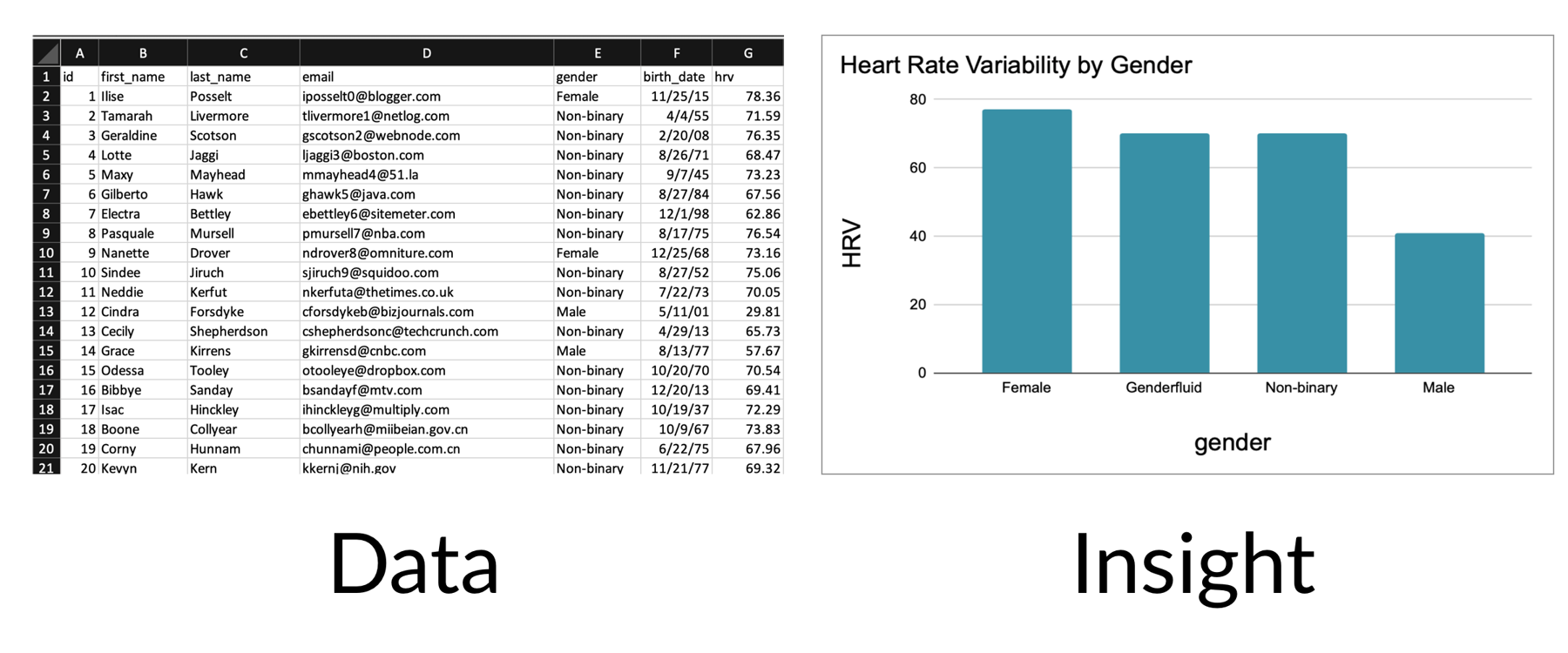
There are many fancy explanations of what insights are. In my opinion, they are gain in knowledge about how something works. In the visualization above, we can see the females score higher than males, and males lower than non-binary genders. This is insight.
Looking at the "Data" pane, little insight can be gained. There is information , such as an email we could use to contact someone. Or their name, by which to address them. However, there isn't anything which explains how something works. These are data.
Unfortunately, in information technology, converting data into insight is tough. As I hope to demonstrate.
Heart Rate Variability
Throughout this article I'm going to use examples regarding Heart Rate Variability . As the name suggests, it is a measure of variability between heart-beats. To be clear, not the time between heart-beats, but the variability .
I find heart rate variability, or HRV, fascinating because it is linked to human stress levels. Research seems to indicate if HRV is high, then you are relaxed. But if your HRV is low, you are stressed. Evolutionarily, this makes sense. During times of stress your heart is one of the most important organs in your body. It focuses up and ensures all muscles and organs are ready for fighting hard or running harder. The famous fight-or-flight. However, during times of relaxation, your heart chills out too. Its beats are less well timed. Hey, your heart works hard!
Not required to follow this article, but if you want to read more about HRV:
I got interested in HRV as I found Apple Watch now tracks it. And I've been curious if it is an actual valid indicator of my stress levels.
What's the Problem?
So what does this have to do with a data warehouses? Let's look at the HRV data the Apple Watch produces.
| occurrence_id | user_id | start | end | hrv |
|---|---|---|---|---|
| 1 | 1 | 2021-09-01 14:10:01 | 2021-09-01 17:00:00 | 40 |
| 2 | 1 | 2021-09-01 19:00:00 | 2021-09-01 23:00:00 | 55 |
| 3 | 1 | 2021-09-02 05:00:00 | 2021-09-03 13:00:01 | 120 |
| 4 | 1 | 2021-09-04 14:00:00 | 65 |
These data have a
start
and
end
time, and if the
end
time is blank it means it is still going. They also have a
user_id
and the
heart_rate_variability
score. Let's try to ask the data a question.
- What is my average HRV per day?
A naive method for querying these data might look like:
  SELECT AVG(heart_rate_variability)   AS avg_hrv,
         COALESCE(DATE(start), DATE('')) AS day
    FROM df
GROUP BY day
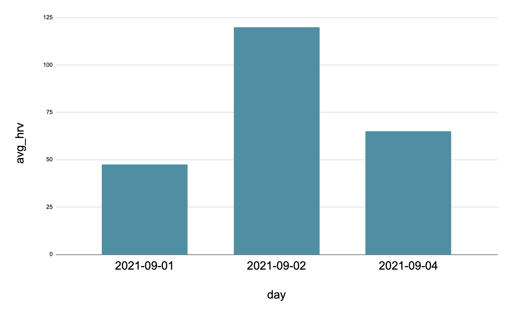
This produces the following:

This looks pretty good. We can get a bit of insight, it looks like my average HRV might be 50. And it looks like
09-02
was an extremely relaxed day. But, what happened to
2021-09-03
?
This is where things start getting complex. There is a long history in databases of converting sustained values to a
start
and
stop
value. Databases are highly optimized for updating records quickly and minimizing the amount of disk space needed to store the data. These types of databases are known as online transactional processing (OLTP) databases. And they are the antithesis of a data warehouse. Data warehouses are known as online analytical processing (OLAP) databases. Unlike OLTP, they are optimized for speed of providing insights. I'll go in more depth about OLTP vs. OLAP a bit later.
Let's get back to solving the problem.
The Infamous Calendar Table
Let's look at what the
start-stop
data actually represent.
| avg_hrv | day |
|---|---|
| 47.5 | 2021-09-01 |
| 65 | 2021-09-02 |
| 65 | 2021-09-03 |
| 120 | 2021-09-04 |
Simple enough, right? But how do we transform the
start
and
stop
data into a list of all dates with sustained values. The most straightforward method is the calendar table.
In SQL, every query must begin with a base table. This is the table associated with the
FROM
keyword. This is the base for all other data are retrieved. In our problem, what we really need is a base table which fills in all the possible missing dates in the
start-stop
data.
In this situation, it is known as a "calendar table" and is simply a list of possible dates you wish to include in your query.
For example:
| date |
|---|
| 2021-09-01 |
| 2021-09-02 |
| 2021-09-03 |
| 2021-09-04 |
Nice! But how do we apply this to our question?
- What is my average HRV per day?
We can apply it with the following query:
   SELECT
          AVG(hrv) avg_hrv,
          c.date
     FROM calendar AS c
LEFT JOIN hrvs AS h
       ON c.date BETWEEN DATE(start)
                     AND COALESCE(DATE(end), DATE('2021-09-05'))
    GROUP BY c.date
This joins all of the HRV
start-stop
values to the
calendar
table where the
calendar.date
falls between the
hrvs.start
and
hrvs.stop
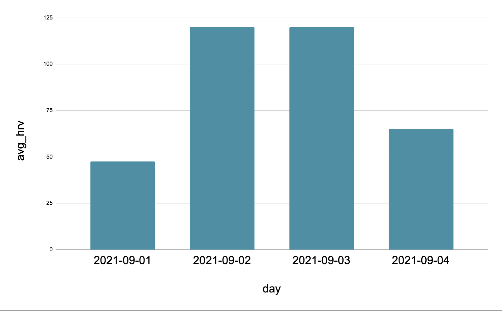
dates. This is the result:

Perfect, this has the exact effect we wish. It expands the
start-stop
dates for all days and calculates the average heart rate variability per day. You may ask, "But this only generated one extra date right? Do we really need a data warehouse for it; can't a classical database solve it?" Yes, yes it can. But! Is it
really
one extra day?
Let's change our question slightly.
- What is my average HRV per hour ?
Some of you may see where I'm going here, but let's just draw it out anyway. We can answer the above question with another calendar table, but this one with a finer grain (level of granularity). That is, our calendar table will now have an entry for every hour between the minimum
start
and
maximum
exit.
| date |
|---|
| 2021-09-01 00:00:00 |
| 2021-09-01 01:00:00 |
| 2021-09-01 02:00:00 |
| 2021-09-01 03:00:00 |
| .... |
| 2021-09-04 04:00:00 |
| 2021-09-04 05:00:00 |
| 2021-09-04 06:00:00 |
| 2021-09-04 07:00:00 |
| 2021-09-04 08:00:00 |
Then, we can run the following query:
   SELECT
          AVG(hrv) avg_hrv,
          c.date
     FROM calendar AS c
LEFT JOIN hrvs AS h
       ON c.date BETWEEN start
                     AND COALESCE(end, '2021-09-05 23:59:59')
    GROUP BY c.date
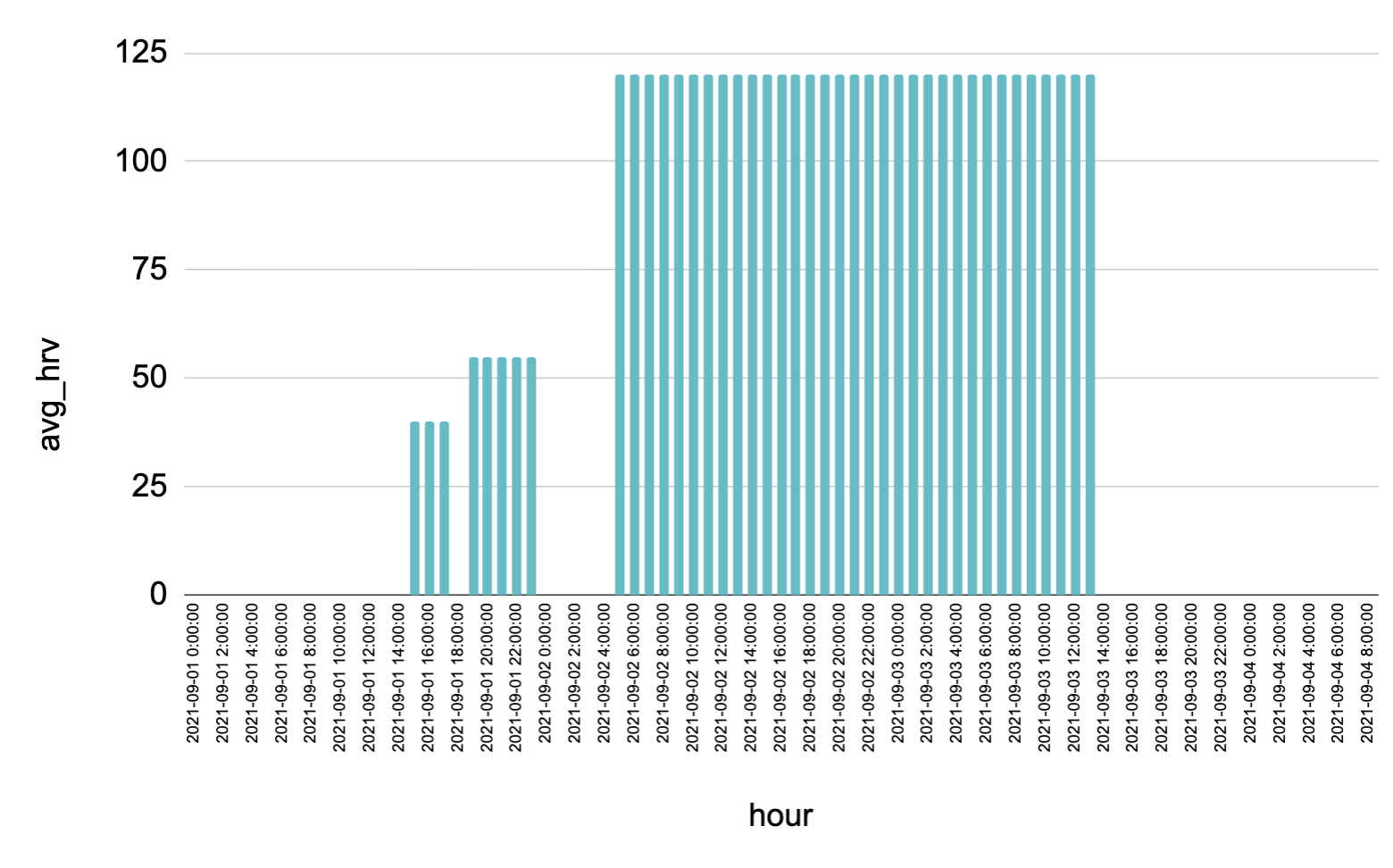
Our result should look something like this:

And here in lies the problem. When we begin to try and expand the data, they have a tendency to grow in number. These sorts of relationships have all sorts of terms associated with it. In SQL, we refer to the relationship having a
one-to-many
or
many-to-many
relationship. That is, one or more dates in the
calendar
table refer to many
start-stop
entries in the
hrv
table. And when the result increases greatly due to a join, we refer to this as "fan out."
Just One More
At this point you may be wondering if this calendar table was really the best way to answer the questions we have. Well, I'm going to risk boring you by giving you just a few more examples.
Let's say you want to ask the data:
- What is average HRV of everyone per hour? :exploding_head:
This would take data like this:
| occurrence_id | user_id | start | end | heart_rate_variability |
|---|---|---|---|---|
| 1 | 1 | 2021-09-01 14:10:01 | 2021-09-01 17:00:00 | 40 |
| 2 | 1 | 2021-09-01 19:00:00 | 2021-09-01 23:00:00 | 55 |
| 3 | 1 | 2021-09-02 5:00:00 | 2021-09-02 13:00:01 | 120 |
| 4 | 1 | 2021-09-02 14:00:00 | 65 | |
| 5 | 2 | 2021-09-01 8:00:00 | 2021-09-01 17:00:00 | 80 |
| 6 | 2 | 2021-09-01 18:00:00 | 2021-09-01 22:00:00 | 35 |
| 7 | 2 | 2021-09-02 5:30:00 | 2021-09-02 17:00:00 | 25 |
| 8 | 2 | 2021-09-02 17:00:00 | 105 |
And join it to the calendar table. The math, roughly, works out to something like this.
[minutes between min and max dates] x [users] = [rows of data]
And to make it even more apparent, what if we ask something like:
- What is average HRV of everyone per minute?
2 user x 365 days x 24 hours x 60 minute = 1,051,200
For 5 users?
5 user x 525,600 minute = 2,628,000
100?
100 user x 525,600 minute = 52,560,000
This sheer number of rows of data which must be processed is the reason for a data warehouse.
OLTP
Let's examine Online Transactional Processing databases to understand why they have difficulty with reading large number of rows. First, what exactly are we talking about when we say "an OLTP database"? In the wild, most database technologies are OLTP, as they fit the most common need of a database.
For example,
There are many, many more.
A clever individual may argue, "Wait, these database technologies are capable of being setup as an OLAP database." True, many of the above have "plugins" or settings to allow them to act as an analytics database, however, their primary purpose is transactional processing. This leads us to the question, "What is 'transactional processing' anyway?"
Don't let the name try to trick you. Transactional processing databases are exactly how they sound. They are technologies optimized for large amounts of small transactions. These transactions may be retrieving a username, then updating a service entry. Or retrieving a user ID, then adding an address. But most involve at least one read and write operation, thus "transaction." These transactions are usually extremely short and involve a small amount of data. Let's go through the details of the characteristics a bit more.
Supports Large Amounts of Concurrency
OLTP DBs are designed for large amounts of users making short queries of the database. This makes them perfect for the backend of many software applications. Let's take a small online bookstore called Amazingzone. This bookstore will often have 300 or so customers interacting with their webpage at a time.
Each time they click on a product the web application sends a query to the
products
table and retrieves the product information. Then, it updates a record in the
visitor
table indicating a user viewed a product. Given each customer is casually browsing, this may lead to a few thousand queries a minute. Each query would look something like this:
SELECT product_name, product_image_path
  FROM products
 WHERE id = 534;
 INSERT user_id, view_date INTO visitors VALUES (754, CURRENT_DATE());
Even though though there are thousands of queries a minute, each one is retrieving a single record, from a single table. This is what is meant when you see a database which is "optimized for concurrency." It means the database is designed to allow thousands of small queries to be executed simultaneously.
Data are Normalized
Another characteristic of an OLTP database is the data are often normalized into at least the 2rd Normal Form . An oversimplified explanation would be: "More tables, less data."
One of the goals of normalization is to reduce the amount of disk space a database needs. This comes from an age where databases were limited to kilobytes of data rather than exabytes. With that in mind, for the following example let's assume every cell beside the field headers require 1 byte regardless of the datatype or information contained.
| id | avg_hrv | date | user_id | user_name | user_age |
|---|---|---|---|---|---|
| 0 | 47.5 | 2021-09-01 | 1 | Thomas | 41 |
| 1 | 120 | 2021-09-02 | 1 | Thomas | 41 |
| 2 | 120 | 2021-09-03 | 1 | Thomas | 41 |
| 3 | 65 | 2021-09-04 | 1 | Thomas | 41 |
Given the table above, it would take 24 bytes to store all the information on a database. If our goal is reducing disk space, 2nd Normal Form (2NF) can help. Let's see what these same data look like after "normalization."
We will split the data into two tables,
hrv_recordings
and
users
.
Here's the
hrv_recordings
table:
| id | avg_hrv | date | user_id |
|---|---|---|---|
| 0 | 47.5 | 2021-09-01 | 1 |
| 1 | 120 | 2021-09-02 | 1 |
| 2 | 120 | 2021-09-03 | 1 |
| 3 | 65 | 2021-09-04 | 1 |
And the
users
table:
| id | user_name | user_age |
|---|---|---|
| 1 | Thomas | 41 |
Now we have two tables joined by the
id
of the user's table, the
Primary Key
, and the
user_id
in the
hrv_recordings
table, the
Foreign Key
. When we query these data we can put the tables back together by using the
JOIN
keyword.
For example:
SELECT *
  FROM hrv_recordings AS hrvr
  JOIN users AS u
    ON hrvr.user_id = u.user_id
But why should we normalize these data in the first place. Well, if you go back and count the number of cells after normalization you will find their are 19. For our oversimplified scenario, that means we have saved 5 bytes through normalization! Pretty nifty.
And if 5 bytes doesn't seem impressive, change it to a percentage. This represents a 20% savings. Let's say your database is 100 GBs and our normalization savings scale linearly. The means you saved 20 GBs simply by changing how your data are stored! Nice job, you.
But the skeptics may be curious at about the catch. Well, the catch is the one reason normalized databases aren't great for analytics. Normalization optimizes for reduced disk space needed and quick inserts, not how quickly the data can be read.
Going back to the SQL query:
SELECT *
  FROM hrv_recordings AS hrvr
  JOIN users AS u
    ON hrvr.user_id = u.user_id
What's really happening in this join can be simplified into a comparison loop.
For example:
for i in range(hrv_recordings.shape[0]):
  for j in range(users.shape[0]):
    if hrv_recordings[i:i+1,0] == users[j:j+1,0]:
      return (hrv_recordings[i:i+1,:], users[j:j+1,:])
If the above Python snippet doesn't make sense, ignore it. Just know joins in SQL come with a computation cost every time a query is executed. And that's the primary trade off with normalization, you are reducing the amount of disk space needed to store the data at the cost of retrieving the data quickly.
Row Based
One of the greatest tricks of OLTPs is stored data in a row object. What does that mean? Let's look at an example.
| id | hrv | date | user_id | user_name | user_age |
|---|---|---|---|---|---|
| 1 | 47.5 | 2021-09-01 | 1 | Thomas | 41 |
| 2 | 120 | 2021-09-02 | 1 | Thomas | 41 |
| 3 | 120 | 2021-09-03 | 1 | Thomas | 41 |
| 4 | 65 | 2021-09-04 | 1 | Thomas | 41 |
Consider the data above. This is how they when you query the database, but how are they actually stored on the database? Well, they are stored in objects based on the row. For example, the above would be stored in text file something like
(1,47.5,2021-09-01,1,Thomas,41)
(2,120,2021-09-02,1,Thomas,41)
(3,120,2021-09-03,1,Thomas,41)
(4,65,2021-09-04,1,Thomas,41)
Each of the rows are an object. This actually gives huge benefits for a transactional database.
Take adding a new record for example, we could send the following to the database.
INSERT INTO hrv_recordings VALUES (70,"2021-09-05","Thomas", 55)
After execution, the database would like this:
(1,47.5,2021-09-01,1,Thomas,41)
(2,120,2021-09-02,1,Thomas,41)
(3,120,2021-09-03,1,Thomas,41)
(4,65,2021-09-04,1,Thomas,41)
(5,70,2021-09-05,Thomas, 41)
Note, the first value is the primary key and we will assume it automatically increments by 1 on every inserts into the table.
Ok, so what's the big deal? A lot actually. The insert did not need to move around any other data to be inserted. That is, row 1-4 were completely untouched. They didn't need to be moved. They didn't need to be updated. Nothing. The advantage of this for transactional databases really only becomes apparent when you compare it to a database which stores data as a column.
Let's take the same data and setup it up to be stored in columns
Here is how those same data would look if stored as column objects. And now, to insert the same data we would need to open the
id
column, insert the new value. Open the
hrv
column and insert the new value and resave it. And so forth.
(1,2,3,4)
(47,120,120,65)
(2021-09-01,2021-09-02,2021-09-03,2021-09-04)
(Thomas,Thomas,Thomas,Thomas)
(41,41,41,41)
This means, for the same insert, we have to do 5 inserts. Each one of these actions is blazing fast, but still, not as fast the row based insert which only took 1 insert action.
Fast Inserts, Updates, Upserts
Now we have talked about normalized and row based data structures, we can now see what "optimized for writing" means.
Let's revisit the normalized data structure. We have two small normalized tables,
hrv_recordings
and
users
.
Here's the
hrv_recordings
table:
| id | avg_hrv | date | user_id |
|---|---|---|---|
| 0 | 47.5 | 2021-09-01 | 1 |
| 1 | 120 | 2021-09-02 | 1 |
| 2 | 120 | 2021-09-03 | 1 |
| 3 | 65 | 2021-09-04 | 1 |
And the
users
table:
| id | user_name | user_age |
|---|---|---|
| 1 | Thomas | 41 |
Let's say a new user signs up, given this is a row based database and the data are broken into separate tables, we can add a user simply by inserting one row in the
users
table.
That is, to insert
Jane
who is
25
, we would simply add a row at the end.
(Thomas,41)
(Jane,25)
We don't need to add any rows to other tables, as Jane did not come into the system with any data.
Now, if the data were not normalized, we'd have to update this table
| id | hrv | date | user_id | user_name | user_age |
|---|---|---|---|---|---|
| 1 | 47.5 | 2021-09-01 | 1 | Thomas | 41 |
| 2 | 120 | 2021-09-02 | 1 | Thomas | 41 |
| 3 | 120 | 2021-09-03 | 1 | Thomas | 41 |
| 4 | 65 | 2021-09-04 | 1 | Thomas | 41 |
With the following row:
(NULL,NULL,Jane,25)
And the resulting table would be:
(1,47.5,2021-09-01,1,Thomas,41)
(2,120,2021-09-02,1,Thomas,41)
(3,120,2021-09-03,1,Thomas,41)
(4,65,2021-09-04,1,Thomas,41)
(5,NULL,NULL,Jane,25)
But this is wasteful, as there is no reason to insert
NULL
s.
OLAPs in Judgement
Let's Talk Rows and Columns
As the name suggests, MariaDB ColumnStore stores the data in column format. This is referred to a columnar database management system (CDBMS). They differ from the row based database management system (RDBMS) in how they store data. There is lots of history on why, but historically, the world has used RDBMS to store data.
You can think of CDBMS and RDBMS as tools for specific jobs. They both work with data, but they have pros and cons which must be assessed when applying them.
Here is my summary comparison of the two systems.
